How to Blur Filters in OpenCV

This demonstration will introduce how to smooth or blur images in OpenCV. We will discuss different types of blur filters and how to use them at the end of this article.

Use Different Types of Blur Filters in OpenCV

Smoothing, also known as blurring, is one of the most commonly used operations in image processing. It is commonly used to remove noise from images.

We can use diverse linear filters because linear filters are easy to achieve and relatively fast. There are various kinds of filters available in OpenCV, for example, homogeneous, Gaussian, median, or bilateral filters, which we will see individually.

First of all, we will see the homogeneous filter. The homogeneous filter is simple, and each output pixel is the mean of its kernel neighbors in a homogeneous filter.

All pixels contribute with an equal weight which is why they are called homogeneous filters. In other words, the kernel is a shape we can apply or convolve over an image.

The numpy creates this kind of squared kernel. So in a homogeneous filter, the kernel looks like this image.

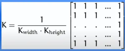
In the homogeneous filter, the kernel K equals 1 divided by the kernel’s width multiplied by the kernel’s height. If we want to use a kernel of 5 by 5 using this formula, then we will have K equals 1 divided by 25, and we will have a 5 by 5 kernel matrix of 1s.

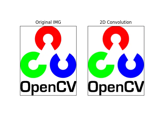
Now, we need to create this kernel for the image filtering using filter2D() or the homogeneous filter. First, we will read an image using the imread() method.

IMG = cv2.imread("opencv-logo.jpg")

We need to convert the image from BGR to RGB because matplotlib reads the images in the RGB format, and OpenCV reads the images in BGR format.

IMG = cv2.cvtColor(IMG, cv2.COLOR_BGR2RGB)

We need to define a 5x5 kernel using the ones() method with the float32 data type, and we will divide it by 25.

K = np.ones((5, 5), np.float32) / 25

Now, we can define our destination image by assisting the defined kernel. A method called filter2D() is used for the homogeneous filter.

The first parameter will be the source image, the second is the desired depth of the destination image, and the third is the kernel.

HMG = cv2.filter2D(IMG, -1, K)

In the next line, we are iterating a for loop, and we will show images on matplotlib in 1 by 2 format through this loop.

for j in range(2):
    plot.subplot(1, 2, j + 1), plot.imshow(IMGS[j], "gray")

Complete example source code:

import numpy as np
import matplotlib.pyplot as plot

IMG = cv2.imread("opencv-logo.jpg")
IMG = cv2.cvtColor(IMG, cv2.COLOR_BGR2RGB)

K = np.ones((5, 5), np.float32) / 25
HMG = cv2.filter2D(IMG, -1, K)


T = ["Original IMG", "2D Convolution"]
IMGS = [IMG, HMG]

for j in range(2):
    plot.subplot(1, 2, j + 1), plot.imshow(IMGS[j], "gray")
    plot.title(T[j])
    plot.xticks([]), plot.yticks([])

plot.show()

We can see a little noise in the corners, and after applying the 2D convolution over this image, the corners are slightly smoothed or blurred. The noises are removed or suppressed by this blurring, so this is one way to blur an image using the filter2D() method.

Blur Filter

One-dimensional images can be filtered with low-pass filters or high-pass filters. The low-pass filter helps remove the noise or blurring of the image, etc., and the high-pass filter helps find edges in the images.

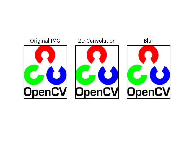
To achieve a blurred image, you need to convert the image with the low pass filter. Various kinds of algorithms are available in OpenCV; the first algorithm is the blur() method.

The blur() method is also called the averaging method, which we will use to apply the averaging algorithm to make the blurred image. This method takes two parameters: the first is the image, and the second is the kernel, which will be (5,5).

import cv2
import numpy as np
import matplotlib.pyplot as plot

IMG = cv2.imread("opencv-logo.jpg")
IMG = cv2.cvtColor(IMG, cv2.COLOR_BGR2RGB)

K = np.ones((5, 5), np.float32) / 25
HMG = cv2.filter2D(IMG, -1, K)
BL = cv2.blur(IMG, (5, 5))

T = ["Original IMG", "2D Convolution", "Blur"]
IMGS = [IMG, HMG, BL]

for j in range(3):
    plot.subplot(1, 3, j + 1), plot.imshow(IMGS[j], "gray")
    plot.title(T[j])
    plot.xticks([]), plot.yticks([])

plot.show()

The result, more or less, looks the same between 2D convolution and blur because we have applied the same kind of kernel to both functions.

Gaussian Filter

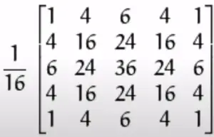
Let’s see the next algorithm, which is the Gaussian filter algorithm. The Gaussian filter is nothing but using a different-weight-kernel in both x and y directions.

In the output, the pixels are located in the middle of the kernel with a higher or bigger weight. The weights decrease with distance from the neighborhood center.

The smaller-weight pixels are located on the side, and the higher-weight pixels are located in the center.

When we take a 5x5 kernel, its result will look like the one shown in the image.

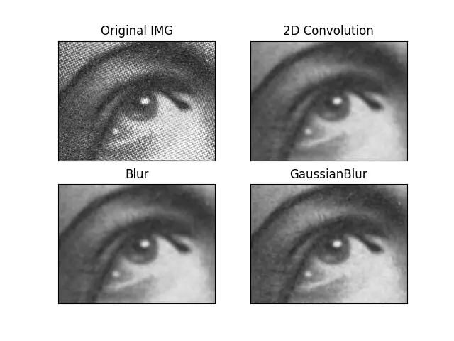
Let’s see how we can use the GaussianBlur() method in OpenCV. The parameters are the same as the blur() method, so the first parameter is the input image, the second one is our kernel, and the third is the Sigma X value.

import cv2
import numpy as np
import matplotlib.pyplot as plot

IMG = cv2.imread("eye.jpg")
IMG = cv2.cvtColor(IMG, cv2.COLOR_BGR2RGB)

K = np.ones((5, 5), np.float32) / 25
HMG = cv2.filter2D(IMG, -1, K)
BL = cv2.blur(IMG, (5, 5))
GB = cv2.GaussianBlur(IMG, (5, 5), 0)

T = ["Original IMG", "2D Convolution", "Blur", "GaussianBlur"]
IMGS = [IMG, HMG, BL, GB]

for j in range(4):
    plot.subplot(2, 2, j + 1), plot.imshow(IMGS[j], "gray")
    plot.title(T[j])
    plot.xticks([]), plot.yticks([])

plot.show()

We can observe that the GaussianBlur() method result is better than the other blurring methods.

Look at the original image, which has too much noise. All noise is removed after applying the GaussianBlur() method.

So the GaussianBlur() method is specifically designed for removing the high-frequency noise from an image.

Median Filter

The median filter is something that replaces each pixel value with the median of its neighboring pixel. The medianBlur() method is great when dealing with an image with salt-and-pepper noise.

If you want to know more about the salt-and-pepper noise, follow this link.

We have here an image; some pixels are distorted, some are the white dots or white noise, and some are where the black noise is seen. Because the pixels are distorted like salt, and the black pixels look like pepper, it is called salt-and-pepper noise.

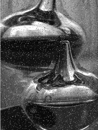
Let’s use this image as a source in the medianBlur() method. The source image will be the first parameter, and the second will be the kernel size.

We must note that the kernel size must be odd, like 3, 5, 7, and so on, except 1. If you use 1, it will show you the original image.

import cv2
import numpy as np
import matplotlib.pyplot as plot

IMG = cv2.imread("water.jpg")
IMG = cv2.cvtColor(IMG, cv2.COLOR_BGR2RGB)

K = np.ones((5, 5), np.float32) / 25
HMG = cv2.filter2D(IMG, -1, K)
BL = cv2.blur(IMG, (5, 5))
GB = cv2.GaussianBlur(IMG, (5, 5), 0)
MB = cv2.medianBlur(IMG, 5)

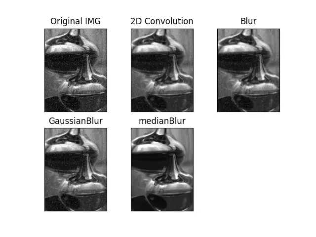
T = ["Original IMG", "2D Convolution", "Blur", "GaussianBlur", "medianBlur"]
IMGS = [IMG, HMG, BL, GB, MB]

for j in range(5):
    plot.subplot(2, 3, j + 1), plot.imshow(IMGS[j], "gray")
    plot.title(T[j])
    plot.xticks([]), plot.yticks([])

plot.show()

We see below the best result we get using the medianBlur() method.

Bilateral Filter

Let’s see the last filter, which is called the bilateral filter. So by using other filters, we not only dissolved the noise but also smoothed the edges.

Sometimes we need to preserve the edges, which means that all the edges remain sharp even if the image is blurred.

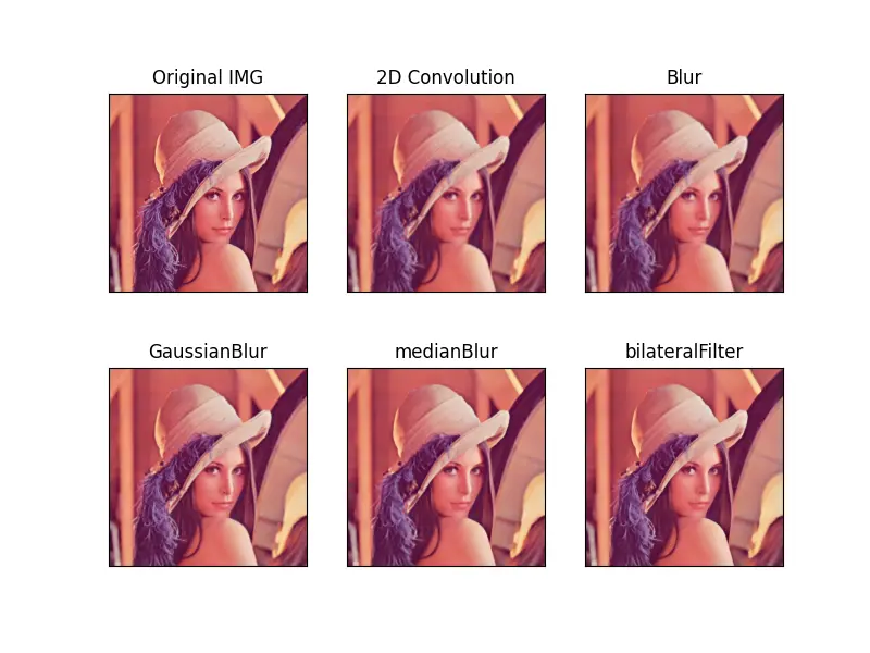
The bilateralFilter() method takes the image as the first parameter. The second parameter is the diameter of each pixel used during the filter, the third parameter is the Sigma color, and the fourth is the Sigma space.

The Sigma color is the filter Sigma in the color space, and Sigma space is the filter Sigma in the coordinate space.

import cv2
import numpy as np
import matplotlib.pyplot as plot

IMG = cv2.imread("lena-1.jpg")
IMG = cv2.cvtColor(IMG, cv2.COLOR_BGR2RGB)

K = np.ones((5, 5), np.float32) / 25
HMG = cv2.filter2D(IMG, -1, K)
BL = cv2.blur(IMG, (5, 5))
GB = cv2.GaussianBlur(IMG, (5, 5), 0)
MB = cv2.medianBlur(IMG, 5)
BF = cv2.bilateralFilter(IMG, 9, 75, 75)

T = [
    "Original IMG",
    "2D Convolution",
    "Blur",
    "GaussianBlur",
    "medianBlur",
    "bilateralFilter",
]
IMGS = [IMG, HMG, BL, GB, MB, BF]
plot.figure(figsize=(8, 6))
for j in range(6):
    plot.subplot(2, 3, j + 1), plot.imshow(IMGS[j], "gray")
    plot.title(T[j])
    plot.xticks([]), plot.yticks([])

plot.show()

Look at how the edges are preserved much better where the bilateralFilter() method is applied. The bilateral filter is highly effective in removing noise while keeping the edges sharp.