How to Create Custom Legend With ggplot in R
-
Use the
legend.positionParameter in thethemeFunction to Specify Legend Position in R -
Use
legend.justificationandlegend.backgroundParameters inthemeFunction to Create Custom Legend -
Use
legend.titleParameter inthemeFunction to Modify Legend Title Formatting
This article will demonstrate multiple methods to create a custom legend with ggplot in R.
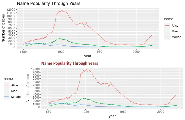
Use the legend.position Parameter in the theme Function to Specify Legend Position in R
The legend.position parameter specifies the legend position in the plot. Optional values can be "none", "left", "right", "bottom", "top" or two-element numeric vector. The plot.title parameter is also utilized in the following example to modify the title of the plot. Finally, two plots are drawn at the same time using the grid.arrange function.
library(ggplot2)
library(gridExtra)
library(babynames)
library(dplyr)

dat <- babynames %>%
  filter(name %in% c("Alice", "Maude", "Mae")) %>%
  filter(sex=="F")

p1 <- ggplot(dat, aes(x = year, y = n, color = name)) +
  geom_line() +
  scale_y_continuous(
    breaks = seq(0, 15000, 1000),
    name = "Number of babies") +
  ggtitle("Name Popularity Through Years")

p2 <- ggplot(dat, aes(x = year, y = n, color = name)) +
  geom_line() +
  scale_y_continuous(
    breaks = seq(0, 15000, 1000),
    name = "Number of babies") +
  theme(
    legend.position = "left",
    plot.title = element_text(
      size = rel(1.2), lineheight = .9,
      family = "Calibri", face = "bold", colour = "brown"
    )) +
  ggtitle("Name Popularity Through Years")

grid.arrange(p1, p2, nrow = 2)
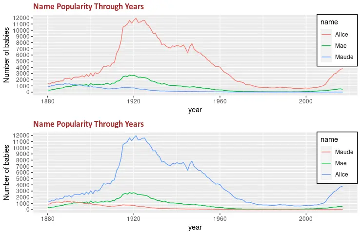
Use legend.justification and legend.background Parameters in theme Function to Create Custom Legend
Another useful parameter of the theme function is legend.background which can be used to format the legend background. The following code snippet fills the legend rectangle with white color and a black stroke. Also, legend.justification is combined with legend.position to specify the legend’s position.
library(ggplot2)
library(gridExtra)
library(babynames)
library(dplyr)

dat <- babynames %>%
  filter(name %in% c("Alice", "Maude", "Mae")) %>%
  filter(sex=="F")

p3 <- ggplot(dat, aes(x = year, y = n, color = name)) +
  geom_line() +
  scale_y_continuous(
    breaks = seq(0, 15000, 1000),
    name = "Number of babies") +
  theme(
    legend.position = c(1, 1),
    legend.justification = c(1, 1),
    legend.background = element_rect(fill = "white", colour = "black"),
    plot.title = element_text(
      size = rel(1.2), lineheight = .9,
      family = "Calibri", face = "bold", colour = "brown"
    )) +
  ggtitle("Name Popularity Through Years")


p4 <- ggplot(dat, aes(x = year, y = n, color = name)) +
  geom_line() +
  scale_color_discrete(limits = c("Maude", "Mae", "Alice")) +
  scale_y_continuous(
    breaks = seq(0, 15000, 1000),
    name = "Number of babies") +
  theme(
    legend.position = c(1, 1),
    legend.justification = c(1, 1),
    legend.background = element_rect(fill = "white", colour = "black"),
    plot.title = element_text(
      size = rel(1.2), lineheight = .9,
      family = "Calibri", face = "bold", colour = "brown"
    )) +
  ggtitle("Name Popularity Through Years")

grid.arrange(p3, p4, nrow = 2)
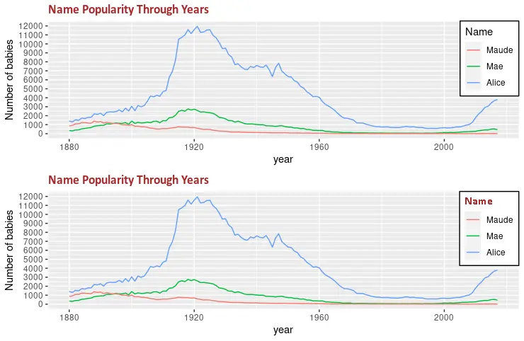
Use legend.title Parameter in theme Function to Modify Legend Title Formatting
The legend.title parameter can be utilized to change the legend title formatting. It takes the element_text function with different arguments to modify the formatting like font family, the color of text, or font size. The grid.arrange function is used to demonstrate the change between the two drawn graphs.
library(ggplot2)
library(gridExtra)
library(babynames)
library(dplyr)

dat <- babynames %>%
  filter(name %in% c("Alice", "Maude", "Mae")) %>%
  filter(sex=="F")

p5 <- ggplot(dat, aes(x = year, y = n, color = name)) +
  geom_line() +
  scale_color_discrete(limits = c("Maude", "Mae", "Alice")) +
  labs(color = "Name") +
  scale_y_continuous(
    breaks = seq(0, 15000, 1000),
    name = "Number of babies") +
  theme(
    legend.position = c(1, 1),
    legend.justification = c(1, 1),
    legend.background = element_rect(fill = "white", colour = "black"),
    plot.title = element_text(
      size = rel(1.2), lineheight = .9,
      family = "Calibri", face = "bold", colour = "brown"
    )) +
  ggtitle("Name Popularity Through Years")


p6 <- ggplot(dat, aes(x = year, y = n, color = name)) +
  geom_line() +
  scale_color_discrete(limits = c("Maude", "Mae", "Alice")) +
  labs(color = "Name") +
  scale_y_continuous(
    breaks = seq(0, 15000, 1000),
    name = "Number of babies") +
  theme(
    legend.title = element_text(
      family = "Calibri",
      colour = "brown",
      face = "bold",
      size = 12),
    legend.position = c(1, 1),
    legend.justification = c(1, 1),
    legend.background = element_rect(fill = "white", colour = "black"),
    plot.title = element_text(
      size = rel(1.2), lineheight = .9,
      family = "Calibri", face = "bold", colour = "brown"
    )) +
  ggtitle("Name Popularity Through Years")

grid.arrange(p5, p6, nrow = 2)

Founder of DelftStack.com. Jinku has worked in the robotics and automotive industries for over 8 years. He sharpened his coding skills when he needed to do the automatic testing, data collection from remote servers and report creation from the endurance test. He is from an electrical/electronics engineering background but has expanded his interest to embedded electronics, embedded programming and front-/back-end programming.
LinkedIn Facebook