Crie uma legenda personalizada com ggplot em R
-
Use o parâmetro
legend.positionna funçãothemepara especificar a posição da legenda em R -
Use os parâmetros
legend.justificationelegend.backgroundna funçãothemepara criar legenda personalizada -
Use o parâmetro
legend.titlena funçãothemepara modificar a formatação do título da legenda
Este artigo demonstrará vários métodos para criar uma legenda personalizada com ggplot em R.
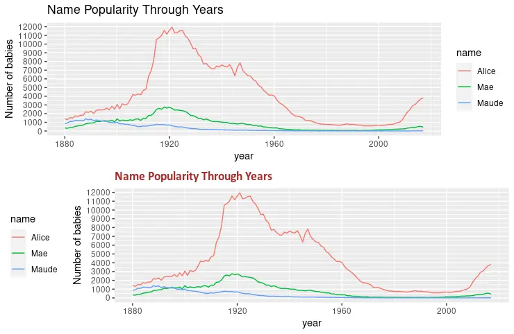
Use o parâmetro legend.position na função theme para especificar a posição da legenda em R
O parâmetro legend.position especifica a posição da legenda no gráfico. Os valores opcionais podem ser "none", "left", "right", "bottom", "top" ou vetor numérico de dois elementos. O parâmetro plot.title também é utilizado no exemplo a seguir para modificar o título do gráfico. Finalmente, dois gráficos são desenhados ao mesmo tempo usando a função grid.arrange.
library(ggplot2)
library(gridExtra)
library(babynames)
library(dplyr)

dat <- babynames %>%
  filter(name %in% c("Alice", "Maude", "Mae")) %>%
  filter(sex=="F")

p1 <- ggplot(dat, aes(x = year, y = n, color = name)) +
  geom_line() +
  scale_y_continuous(
    breaks = seq(0, 15000, 1000),
    name = "Number of babies") +
  ggtitle("Name Popularity Through Years")

p2 <- ggplot(dat, aes(x = year, y = n, color = name)) +
  geom_line() +
  scale_y_continuous(
    breaks = seq(0, 15000, 1000),
    name = "Number of babies") +
  theme(
    legend.position = "left",
    plot.title = element_text(
      size = rel(1.2), lineheight = .9,
      family = "Calibri", face = "bold", colour = "brown"
    )) +
  ggtitle("Name Popularity Through Years")

grid.arrange(p1, p2, nrow = 2)
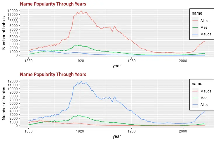
Use os parâmetros legend.justification e legend.background na função theme para criar legenda personalizada
Outro parâmetro útil da função theme é legend.background que pode ser usado para formatar o fundo da legenda. O trecho de código a seguir preenche o retângulo da legenda com a cor branca e um traço preto. Além disso, legend.justification é combinado com legend.position para especificar a posição da legenda.
library(ggplot2)
library(gridExtra)
library(babynames)
library(dplyr)

dat <- babynames %>%
  filter(name %in% c("Alice", "Maude", "Mae")) %>%
  filter(sex=="F")

p3 <- ggplot(dat, aes(x = year, y = n, color = name)) +
  geom_line() +
  scale_y_continuous(
    breaks = seq(0, 15000, 1000),
    name = "Number of babies") +
  theme(
    legend.position = c(1, 1),
    legend.justification = c(1, 1),
    legend.background = element_rect(fill = "white", colour = "black"),
    plot.title = element_text(
      size = rel(1.2), lineheight = .9,
      family = "Calibri", face = "bold", colour = "brown"
    )) +
  ggtitle("Name Popularity Through Years")


p4 <- ggplot(dat, aes(x = year, y = n, color = name)) +
  geom_line() +
  scale_color_discrete(limits = c("Maude", "Mae", "Alice")) +
  scale_y_continuous(
    breaks = seq(0, 15000, 1000),
    name = "Number of babies") +
  theme(
    legend.position = c(1, 1),
    legend.justification = c(1, 1),
    legend.background = element_rect(fill = "white", colour = "black"),
    plot.title = element_text(
      size = rel(1.2), lineheight = .9,
      family = "Calibri", face = "bold", colour = "brown"
    )) +
  ggtitle("Name Popularity Through Years")

grid.arrange(p3, p4, nrow = 2)
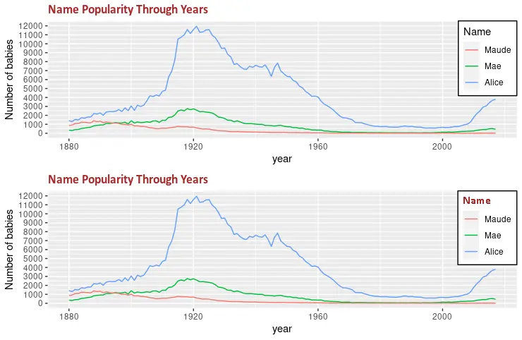
Use o parâmetro legend.title na função theme para modificar a formatação do título da legenda
O parâmetro legend.title pode ser utilizado para alterar a formatação do título da legenda. É necessária a função element_text com diferentes argumentos para modificar a formatação, como família de fontes, cor do texto ou tamanho da fonte. A função grid.arrange é usada para demonstrar a mudança entre os dois gráficos desenhados.
library(ggplot2)
library(gridExtra)
library(babynames)
library(dplyr)

dat <- babynames %>%
  filter(name %in% c("Alice", "Maude", "Mae")) %>%
  filter(sex=="F")

p5 <- ggplot(dat, aes(x = year, y = n, color = name)) +
  geom_line() +
  scale_color_discrete(limits = c("Maude", "Mae", "Alice")) +
  labs(color = "Name") +
  scale_y_continuous(
    breaks = seq(0, 15000, 1000),
    name = "Number of babies") +
  theme(
    legend.position = c(1, 1),
    legend.justification = c(1, 1),
    legend.background = element_rect(fill = "white", colour = "black"),
    plot.title = element_text(
      size = rel(1.2), lineheight = .9,
      family = "Calibri", face = "bold", colour = "brown"
    )) +
  ggtitle("Name Popularity Through Years")


p6 <- ggplot(dat, aes(x = year, y = n, color = name)) +
  geom_line() +
  scale_color_discrete(limits = c("Maude", "Mae", "Alice")) +
  labs(color = "Name") +
  scale_y_continuous(
    breaks = seq(0, 15000, 1000),
    name = "Number of babies") +
  theme(
    legend.title = element_text(
      family = "Calibri",
      colour = "brown",
      face = "bold",
      size = 12),
    legend.position = c(1, 1),
    legend.justification = c(1, 1),
    legend.background = element_rect(fill = "white", colour = "black"),
    plot.title = element_text(
      size = rel(1.2), lineheight = .9,
      family = "Calibri", face = "bold", colour = "brown"
    )) +
  ggtitle("Name Popularity Through Years")

grid.arrange(p5, p6, nrow = 2)

Founder of DelftStack.com. Jinku has worked in the robotics and automotive industries for over 8 years. He sharpened his coding skills when he needed to do the automatic testing, data collection from remote servers and report creation from the endurance test. He is from an electrical/electronics engineering background but has expanded his interest to embedded electronics, embedded programming and front-/back-end programming.
LinkedIn Facebook