How to Implement Gradient Descent Using NumPy and Python

1. Gradient Descent
2. Implementation of Gradient Descent Using Python

Machine Learning is a trend these days. Every company or startup is trying to come up with solutions that use machine learning to solve real-world problems. To solve these problems, programmers build machine learning models trained over some essential and valuable data. While training models, there are many tactics, algorithms, and methods to choose from. Some might work, and some would not.

Generally, Python is used to train these models. Python has support for numerous libraries that make it easy to implement machine learning concepts. One such concept is gradient descent. In this article, we will learn how to implement gradient descent using Python.

Gradient Descent

Gradient Descent is a convex function-based optimization algorithm that is used while training the machine learning model. This algorithm helps us find the best model parameters to solve the problem more efficiently. While training a machine learning model over some data, this algorithm tweaks the model parameters for each iteration which finally yields a global minima, sometimes even a local minima, for the differentiable function.

While tweaking the model parameters, a value known as the learning rate decides the amount by which the values should be tweaked. If this value is too large, the learning will be fast, and we might end up underfitting the model. And, if this value is too small, the learning will be slow, and we might end up overfitting the model to the training data. Hence, we have to come up with a value that maintains a balance and finally yields a good machine learning model with good accuracy.

Implementation of Gradient Descent Using Python

Now that we are done with the brief theory of gradient descent, let us understand how we can implement it with the help of the NumPy module and Python programming language with the help of an example.

We will train a machine learning model for the equation y = 0.5x + 2, which is of the form y = mx + c or y = ax + b. Essentially will train a machine learning model over the data generated using this equation. The model will guess the values of m and c or a and b, that is, the slope and the intercept, respectively. Since machine learning models need some data to learn from and some testing data to test their accuracy, we will generate the same using a Python script. We will perform linear regression to perform this task.

The training inputs and testing inputs will be in the following form; a two-dimensional NumPy array. In this example, the input is a single integer value, and output is a single integer value. Since a single input can be an array of integer and float values, the following format will be used to promote the reusability of code or dynamic nature.

[[1], [2], [3], [4], [5], [6], [7], ...]

And the training labels and testing labels will be in the following form; a one-dimensional NumPy array.

[1, 4, 9, 16, 25, 36, 49, ...]

Python Code

Following is the implementation of the above example.

import random
import numpy as np
import matplotlib.pyplot as plt


def linear_regression(inputs, targets, epochs, learning_rate):
    """
    A utility function to run linear regression and get weights and bias
    """
    costs = []  # A list to store losses at each epoch
    values_count = inputs.shape[1]  # Number of values within a single input
    size = inputs.shape[0]  # Total number of inputs
    weights = np.zeros((values_count, 1))  # Weights
    bias = 0  # Bias

    for epoch in range(epochs):
        # Calculating the predicted values
        predicted = np.dot(inputs, weights) + bias
        loss = predicted - targets  # Calculating the individual loss for all the inputs
        d_weights = np.dot(inputs.T, loss) / (2 * size)  # Calculating gradient
        d_bias = np.sum(loss) / (2 * size)  # Calculating gradient
        weights = weights - (learning_rate * d_weights)  # Updating the weights
        bias = bias - (learning_rate * d_bias)  # Updating the bias
        cost = np.sqrt(
            np.sum(loss ** 2) / (2 * size)
        )  # Root Mean Squared Error Loss or RMSE Loss
        costs.append(cost)  # Storing the cost
        print(
            f"Iteration: {epoch + 1} | Cost/Loss: {cost} | Weight: {weights} | Bias: {bias}"
        )

    return weights, bias, costs


def plot_test(inputs, targets, weights, bias):
    """
    A utility function to test the weights
    """
    predicted = np.dot(inputs, weights) + bias
    predicted = predicted.astype(int)
    plt.plot(
        predicted,
        [i for i in range(len(predicted))],
        color=np.random.random(3),
        label="Predictions",
        linestyle="None",
        marker="x",
    )
    plt.plot(
        targets,
        [i for i in range(len(targets))],
        color=np.random.random(3),
        label="Targets",
        linestyle="None",
        marker="o",
    )
    plt.xlabel("Indexes")
    plt.ylabel("Values")
    plt.title("Predictions VS Targets")
    plt.legend()
    plt.show()


def rmse(inputs, targets, weights, bias):
    """
    A utility function to calculate RMSE or Root Mean Squared Error
    """
    predicted = np.dot(inputs, weights) + bias
    mse = np.sum((predicted - targets) ** 2) / (2 * inputs.shape[0])
    return np.sqrt(mse)


def generate_data(m, n, a, b):
    """
    A function to generate training data, training labels, testing data, and testing inputs
    """
    x, y, tx, ty = [], [], [], []

    for i in range(1, m + 1):
        x.append([float(i)])
        y.append([float(i) * a + b])

    for i in range(n):
        tx.append([float(random.randint(1000, 100000))])
        ty.append([tx[-1][0] * a + b])

    return np.array(x), np.array(y), np.array(tx), np.array(ty)


learning_rate = 0.0001  # Learning rate
epochs = 200000  # Number of epochs
a = 0.5  # y = ax + b
b = 2.0  # y = ax + b
inputs, targets, train_inputs, train_targets = generate_data(300, 50, a, b)
weights, bias, costs = linear_regression(
    inputs, targets, epochs, learning_rate
)  # Linear Regression
indexes = [i for i in range(1, epochs + 1)]
plot_test(train_inputs, train_targets, weights, bias)  # Testing
print(f"Weights: {[x[0] for x in weights]}")
print(f"Bias: {bias}")
print(
    f"RMSE on training data: {rmse(inputs, targets, weights, bias)}"
)  # RMSE on training data
print(
    f"RMSE on testing data: {rmse(train_inputs, train_targets, weights, bias)}"
)  # RMSE on testing data
plt.plot(indexes, costs)
plt.xlabel("Epochs")
plt.ylabel("Overall Cost/Loss")
plt.title(f"Calculated loss over {epochs} epochs")
plt.show()

a Brief Explanation of the Python Code

The code has the following methods implemented.

• linear_regression(inputs, targets, epochs, learning_rate): This function performs the linear regression over the data and returns model weights, model bias, and intermediate costs or losses for each epoch
• plot_test(inputs, targets, weights, bias): This function accepts inputs, targets, weights, and bias and predicts the output for the inputs. Then it will plot a graph to show how close were the model predictions from the actual values.
• rmse(inputs, targets, weights, bias): This function computes and returns root mean squared error for some inputs, weights, bias, and targets or labels.
• generate_data(m, n, a, b): This function generates sample data for the machine learning model to be trained using the equation y = ax + b. It generates the training and testing data. m and n refer to the number of training and testing samples generated, respectively.

Following is the execution flow of the code above.

Output

The Python code will output the model training status to the console for each epoch or iteration. It will be as follows.

...
Iteration: 199987 | Cost/Loss: 0.05856315870190882 | Weight: [[0.5008289]] | Bias: 1.8339454694938624
Iteration: 199988 | Cost/Loss: 0.05856243033468181 | Weight: [[0.50082889]] | Bias: 1.8339475347628937
Iteration: 199989 | Cost/Loss: 0.05856170197651294 | Weight: [[0.50082888]] | Bias: 1.8339496000062387
Iteration: 199990 | Cost/Loss: 0.058560973627402625 | Weight: [[0.50082887]] | Bias: 1.8339516652238976
Iteration: 199991 | Cost/Loss: 0.05856024528735169 | Weight: [[0.50082886]] | Bias: 1.8339537304158708
Iteration: 199992 | Cost/Loss: 0.05855951695635694 | Weight: [[0.50082885]] | Bias: 1.8339557955821586
Iteration: 199993 | Cost/Loss: 0.05855878863442534 | Weight: [[0.50082884]] | Bias: 1.8339578607227613
Iteration: 199994 | Cost/Loss: 0.05855806032154768 | Weight: [[0.50082883]] | Bias: 1.8339599258376793
...

Once the model is trained, the program will test the model and draw a plot with the model predictions and the true values. The plot trained will be similar to the one shown below. Note that since testing data is generated using the random module, random values will be generated on the fly, and hence, the graph shown below will most likely be different from yours.

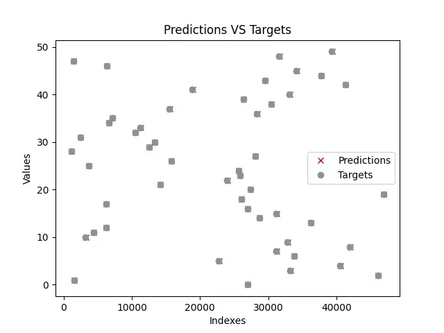
As we can see, the predictions are almost overlapping all the true values (Predictions are represented by x and targets are represented by o). This means that the model has almost successfully predicted the values for a and b or m and c.

Next, the program prints all the losses found while training the model.

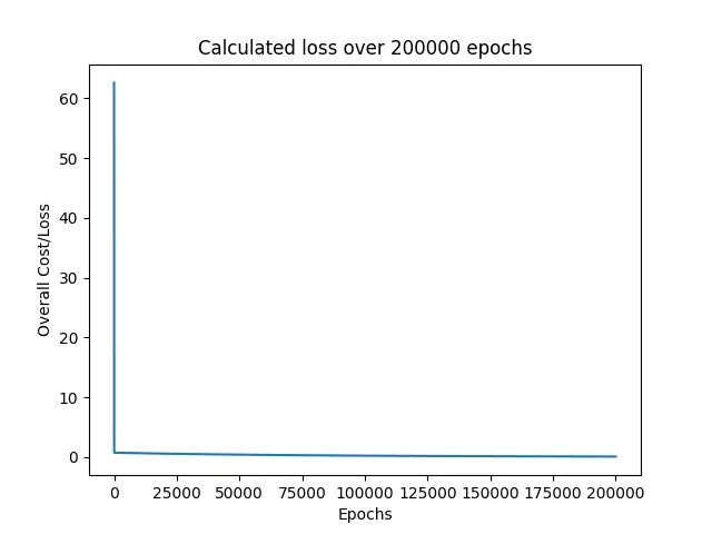
As we can see, the loss immediately fell down from around 60 close to 0 and continued to remain around to it for the rest of the epochs.

Lastly, the RMSE losses for training and testing data were printed, and the predicted values for a and b or the model parameters.

Weights: [0.5008287639956263]
Bias: 1.8339723159878247
RMSE on training data: 0.05855296238504223
RMSE on testing data: 30.609530314187527

The equation that we used for this example was y = 0.5x + 2, where a = 0.5 and b = 2. And, the model predicted a = 0.50082 and b = 1.83397, which are very close to the true values. That is why our predictions were overlapping with the true targets.

For this example, we set the number of epochs to 200000 and the learning rate to 0.0001. Fortunately, this is just one set of configurations that gave us extremely good, almost perfect results. I would highly recommend the readers of this article play around with these values and see if they can come up with some sets of values that yield even better results.