How to Fit Poisson Distribution to Different Datasets in Python

1. Fit Poisson Distribution to Different Datasets in Python
2. Binned Least Squares Method to Fit the Poisson Distribution in Python
3. Use a Negative Binomial to Fit Poisson Distribution Over an Overly Dispersed Dataset
4. Poisson Distribution for Highly Dispersed Data Using Negative Binomial
5. Conclusion

The Poisson probability distribution shows the chance of an event happening in a fixed period or space. This data can be plotted as a histogram using Python to observe the event’s occurrence rate.

Distributions are curves that can be plotted on the histograms or other structures to find the best fit curve for the data set. This article will teach you how to fit Poisson distribution on a data set using Python.

Fit Poisson Distribution to Different Datasets in Python

Let’s understand how to plot multiple distributions on a set of data and fit Poisson distribution using SciPy and Python.

Binned Least Squares Method to Fit the Poisson Distribution in Python

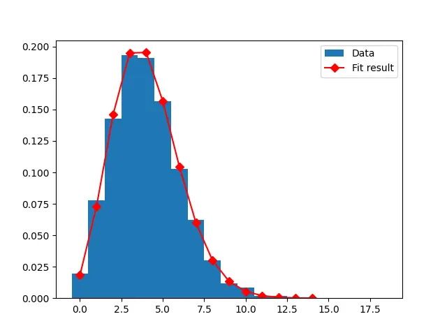
In this example, a dummy Poisson dataset is created, and a histogram is plotted with this data. After the histogram is plotted, the binned least square method fits a curve over the histogram to fit the Poisson distribution.

Import Functions for the Program

This program uses the following import functions.

1. Mathematical arm of Matplotlib - Numpy.
2. The Matplotlib sub-library Pyplot to plot charts.
3. SciPy curve_fit for importing the curve fit.
4. poisson for the dataset.

Create a Dummy Dataset for Poisson Distribution and Plot the Histogram With the Dataset

A variable dataset_size is created with Poisson deviated numbers inside the range of 4-20,000 by using the function np.random.poisson(). It returns an array with random Poisson values.

data_set = np.random.poisson(4, 2000)

The differences in the histogram data are stored inside a new variable, bins. It uses the np.arrange() function to return an array with values between the range of -0.5 to 20 with 0.5 as the mean difference.

bins = np.arange(20) - 0.5

A histogram is plotted using the plt.hist() function, where the parameters are:

1. data_set for the data used.
2. bins for the differences.
3. density, which is set as true.
4. label, which adds a label to the plot.

While the histogram gets plotted, three values are returned from the plt.hist() function, which is stored in three new variables - entries for values of histogram bins, bin_edges for edges of bins, and patches for individual patches for the histogram.

entries, bin_edges, patches = plt.hist(data_set, bins=bins, density=True, label="Data")

Fit the Curve to Histogram Using Curve Fit

Once the histogram is plotted, the curve fit function is used to fit the Poisson distribution to the data. The curve function plots the best fit line from a scattered data set.

The curve fit requires a fit function that converts an array of values into Poisson distribution and returns it as parameters on which the curve will be plotted. A method fit_function is created with two parameters, k and parameters.

The SciPy library poisson.pmf is used to get the parameters. The pmf stands for probability mass function, and this function returns the frequency of a random distribution.

The variable k stores the number of times the event has occured, and the variable lamb is the popt(sum of reduced squares) which is used as the fit parameter for the curve function.

The SciPy curve_fit function takes in three parameters, fit_function, middle_bins, and entries and returns two values - parameters (optimum values that reduce the sum of the square residuals) and cov_matrix (parameters estimated co-variance).

parameters, cov_matrix = curve_fit(fit_function, middles_bins, entries)

A dataset of 15 ascending values is created to plot the curve, and the Poisson distribution of these ascending values is fitted using the fit_function method. The plot’s attributes are provided, and the result is displayed.

x_plot = np.arange(0, 15)

plt.plot(
    x_plot,
    fit_function(x_plot, *parameters),
    marker="D",
    linestyle="-",
    color="red",
    label="Fit result",
)

Complete Code:

import numpy as np
import matplotlib.pyplot as plt
from scipy.optimize import curve_fit
from scipy.stats import poisson

# get random numbers that are poisson deviated
data_set = np.random.poisson(4, 2000)

# the bins have to be kept as a positive integer because poisson is a positive integer distribution
bins = np.arange(20) - 0.5
entries, bin_edges, patches = plt.hist(data_set, bins=bins, density=True, label="Data")

# calculate bin centers
middles_bins = (bin_edges[1:] + bin_edges[:-1]) * 0.5


def fit_function(k, lamb):
    # The parameter lamb will be used as the fit parameter
    return poisson.pmf(k, lamb)


# fit with curve_fit
parameters, cov_matrix = curve_fit(fit_function, middles_bins, entries)

# plot poisson-deviation with fitted parameter
x_plot = np.arange(0, 15)

plt.plot(
    x_plot,
    fit_function(x_plot, *parameters),
    marker="D",
    linestyle="-",
    color="red",
    label="Fit result",
)
plt.legend()
plt.show()

Output:

Use a Negative Binomial to Fit Poisson Distribution Over an Overly Dispersed Dataset

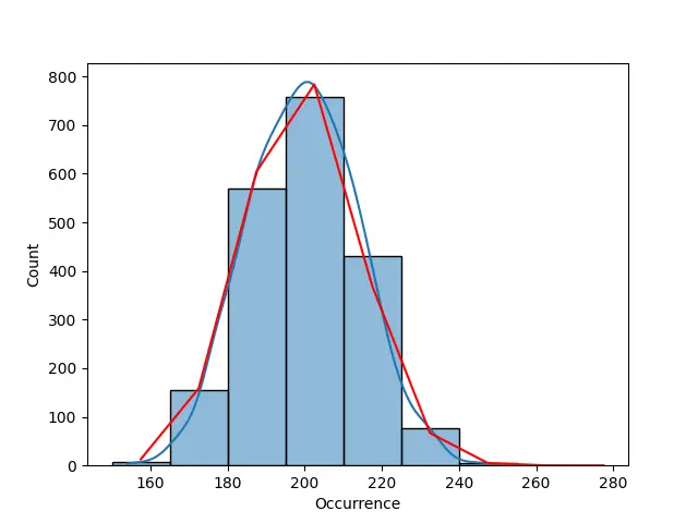
In this example, a Poisson distribution data frame is created with highly dispersed data, and we will learn how to fit Poisson Distribution to this data.

Unlike the last example, where the Poisson distribution was centered around its mean, this data is highly dispersed, so a negative binomial will be added in the next section to this data to improve the Poisson distribution.

Create the Dataset

In this example, a Pandas data frame is created and stored inside the variable dataset. This dataset has one column, Occurrence with 2000 Poisson values and the value of lambda set at 200.

dataset = pd.DataFrame({"Occurrence": np.random.poisson(200, 2000)})

Plot Histogram With the Dataset

To plot the histogram, we need to provide three values, intervals of the bins(bucket of values), the start of bins, and the end of bins. This is done by:

width_of_bin = 15
xstart = 150
xend = 280
bins = np.arange(xstart, xend, width_of_bin)

Once the value of bins is set, plot the histogram.

hist = sns.histplot(data=dataset["Occurrence"], kde=True, bins=bins)

Fit the Poisson Distribution Curve to the Histogram

The mean and size of the dataset are required to fit the Poisson Distribution by plotting the distribution curve. In two new variables, mu and n, the mean and size of the dataset are stored, respectively.

The algorithm to plot the Poisson distribution curve is:

bins + width_of_bin / 2, n * (
    poisson.cdf(bins + width_of_bin, mu) - poisson.cdf(bins, mu)
)

Lastly, the curve is plotted on the histogram.

Complete Code:

import numpy as np
import pandas as pd
import seaborn as sns
import matplotlib.pyplot as plt
from scipy.stats import poisson

dataset = pd.DataFrame({"Occurrence": np.random.poisson(200, 2000)})

width_of_bin = 15
xstart = 150
xend = 280
bins = np.arange(xstart, xend, width_of_bin)

hist = sns.histplot(data=dataset["Occurrence"], kde=True, bins=bins)
mu = dataset["Occurrence"].mean()
n = len(dataset)
plt.plot(
    bins + width_of_bin / 2,
    n * (poisson.cdf(bins + width_of_bin, mu) - poisson.cdf(bins, mu)),
    color="red",
)
plt.show()

Output:

Poisson Distribution for Highly Dispersed Data Using Negative Binomial

As stated earlier, the data inside this dataset is overly dispersed, which is why the curve does not perfectly resemble a Poisson Distribution curve. A negative binomial is used in the example below to fit the Poisson distribution.

The dataset is created by injecting a negative binomial:

dataset = pd.DataFrame({"Occurrence": nbinom.rvs(n=1, p=0.004, size=2000)})

The bin for the histogram starts at 0 and ends at 2000 with a common interval of 100.

binwidth = 100
xstart = 0
xend = 2000
bins = np.arange(xstart, xend, binwidth)

After the bins and dataset are created, the histogram is plotted:

hist = sns.histplot(data=dataset["Occurrence"], kde=True, bins=bins)

The curve requires five parameters, variance(Var), mean(mu), p(mean/variance), r(items taken for consideration), and n(total items in the dataset)

The variance and mean are calculated in two variables, variance and mu.

Var = dataset["Occurrence"].var()
mu = dataset["Occurrence"].mean()

The following formulas are used to find out the p and r:

p = mu / Var
r = mu ** 2 / (Var - mu)

Total numbers of items are stored by saving the length of the dataset in a new variable n.

n = len(dataset)

Lastly, the curve is plotted on the histogram.

plt.plot(
    bins + binwidth / 2,
    n * (nbinom.cdf(bins + binwidth, r, p) - nbinom.cdf(bins, r, p)),
)

Complete Code:

import numpy as np
from scipy.stats import nbinom
import pandas as pd
import seaborn as sns
import matplotlib.pyplot as plt

dataset = pd.DataFrame({"Occurrence": nbinom.rvs(n=1, p=0.004, size=2000)})

binwidth = 100
xstart = 0
xend = 2000
bins = np.arange(xstart, xend, binwidth)

hist = sns.histplot(data=dataset["Occurrence"], kde=True, bins=bins)

Var = dataset["Occurrence"].var()
mu = dataset["Occurrence"].mean()
p = mu / Var
r = mu ** 2 / (Var - mu)
n = len(dataset)

plt.plot(
    bins + binwidth / 2,
    n * (nbinom.cdf(bins + binwidth, r, p) - nbinom.cdf(bins, r, p)),
    color="red",
)
plt.show()

Output:

Conclusion

This article explains three ways to fit a Poisson distribution to a dataset in Python. After reading the article, the reader can fit Poisson distribution over dummy Poisson datasets and overly dispersed datasets.