使用 NumPy 和 Python 实现梯度下降
机器学习是当今的一种趋势。每家公司或初创公司都在尝试提出使用机器学习来解决现实世界问题的解决方案。为了解决这些问题,程序员构建了机器学习模型,这些模型是针对一些重要且有价值的数据进行训练的。在训练模型时,有很多策略、算法和方法可供选择。有些可能会起作用,有些则不会。
通常,使用 Python 来训练这些模型。Python 支持众多库,可以轻松实现机器学习概念。其中一个概念是梯度下降。在本文中,我们将学习如何使用 Python 实现梯度下降。
梯度下降
梯度下降是一种基于凸函数的优化算法,用于训练机器学习模型。该算法帮助我们找到最佳模型参数以更有效地解决问题。在针对某些数据训练机器学习模型时,该算法会为每次迭代调整模型参数,最终为可微函数生成全局最小值,有时甚至是局部最小值。
在调整模型参数时,称为学习率的值决定了应调整值的量。如果这个值太大,学习会很快,我们最终可能会欠拟合模型。而且,如果这个值太小,学习会很慢,我们最终可能会过度拟合模型到训练数据。因此,我们必须提出一个保持平衡的值,并最终产生一个具有良好准确性的良好机器学习模型。
使用 Python 实现梯度下降
现在我们已经完成了梯度下降的简要理论,让我们通过一个例子来了解如何在 NumPy 模块和 Python 编程语言的帮助下实现它。
我们将为方程 y = 0.5x + 2 训练机器学习模型,其形式为 y = mx + c 或 y = ax + b。本质上将针对使用此方程生成的数据训练机器学习模型。模型将分别猜测 m 和 c 或 a 和 b 的值,即斜率和截距。由于机器学习模型需要一些数据来学习和一些测试数据来测试它们的准确性,我们将使用 Python 脚本生成相同的数据。我们将执行线性回归来执行此任务。
训练输入和测试输入将采用以下形式;一个二维 NumPy 数组。在此示例中,输入是单个整数值,输出是单个整数值。由于单个输入可以是整数和浮点值的数组,因此将使用以下格式来提高代码的可重用性或动态性。
[[1], [2], [3], [4], [5], [6], [7], ...]
训练标签和测试标签将采用以下形式;一维 NumPy 数组。
[1, 4, 9, 16, 25, 36, 49, ...]
Python 代码
下面是上面例子的实现。
import random
import numpy as np
import matplotlib.pyplot as plt


def linear_regression(inputs, targets, epochs, learning_rate):
    """
    A utility function to run linear regression and get weights and bias
    """
    costs = []  # A list to store losses at each epoch
    values_count = inputs.shape[1]  # Number of values within a single input
    size = inputs.shape[0]  # Total number of inputs
    weights = np.zeros((values_count, 1))  # Weights
    bias = 0  # Bias

    for epoch in range(epochs):
        # Calculating the predicted values
        predicted = np.dot(inputs, weights) + bias
        loss = predicted - targets  # Calculating the individual loss for all the inputs
        d_weights = np.dot(inputs.T, loss) / (2 * size)  # Calculating gradient
        d_bias = np.sum(loss) / (2 * size)  # Calculating gradient
        weights = weights - (learning_rate * d_weights)  # Updating the weights
        bias = bias - (learning_rate * d_bias)  # Updating the bias
        cost = np.sqrt(
            np.sum(loss ** 2) / (2 * size)
        )  # Root Mean Squared Error Loss or RMSE Loss
        costs.append(cost)  # Storing the cost
        print(
            f"Iteration: {epoch + 1} | Cost/Loss: {cost} | Weight: {weights} | Bias: {bias}"
        )

    return weights, bias, costs


def plot_test(inputs, targets, weights, bias):
    """
    A utility function to test the weights
    """
    predicted = np.dot(inputs, weights) + bias
    predicted = predicted.astype(int)
    plt.plot(
        predicted,
        [i for i in range(len(predicted))],
        color=np.random.random(3),
        label="Predictions",
        linestyle="None",
        marker="x",
    )
    plt.plot(
        targets,
        [i for i in range(len(targets))],
        color=np.random.random(3),
        label="Targets",
        linestyle="None",
        marker="o",
    )
    plt.xlabel("Indexes")
    plt.ylabel("Values")
    plt.title("Predictions VS Targets")
    plt.legend()
    plt.show()


def rmse(inputs, targets, weights, bias):
    """
    A utility function to calculate RMSE or Root Mean Squared Error
    """
    predicted = np.dot(inputs, weights) + bias
    mse = np.sum((predicted - targets) ** 2) / (2 * inputs.shape[0])
    return np.sqrt(mse)


def generate_data(m, n, a, b):
    """
    A function to generate training data, training labels, testing data, and testing inputs
    """
    x, y, tx, ty = [], [], [], []

    for i in range(1, m + 1):
        x.append([float(i)])
        y.append([float(i) * a + b])

    for i in range(n):
        tx.append([float(random.randint(1000, 100000))])
        ty.append([tx[-1][0] * a + b])

    return np.array(x), np.array(y), np.array(tx), np.array(ty)


learning_rate = 0.0001  # Learning rate
epochs = 200000  # Number of epochs
a = 0.5  # y = ax + b
b = 2.0  # y = ax + b
inputs, targets, train_inputs, train_targets = generate_data(300, 50, a, b)
weights, bias, costs = linear_regression(
    inputs, targets, epochs, learning_rate
)  # Linear Regression
indexes = [i for i in range(1, epochs + 1)]
plot_test(train_inputs, train_targets, weights, bias)  # Testing
print(f"Weights: {[x[0] for x in weights]}")
print(f"Bias: {bias}")
print(
    f"RMSE on training data: {rmse(inputs, targets, weights, bias)}"
)  # RMSE on training data
print(
    f"RMSE on testing data: {rmse(train_inputs, train_targets, weights, bias)}"
)  # RMSE on testing data
plt.plot(indexes, costs)
plt.xlabel("Epochs")
plt.ylabel("Overall Cost/Loss")
plt.title(f"Calculated loss over {epochs} epochs")
plt.show()
Python 代码的简要说明
代码实现了以下方法。
linear_regression(inputs, targets, epochs, learning_rate):该函数对数据执行线性回归,并返回每个时期的模型权重、模型偏差和中间成本或损失plot_test(inputs, targets, weights, bias):该函数接受输入、目标、权重和偏差,并预测输入的输出。然后它会绘制一个图表来显示模型预测与实际值的接近程度。rmse(输入、目标、权重、偏差):该函数计算并返回某些输入、权重、偏差和目标或标签的均方根误差。generate_data(m, n, a, b):该函数为机器学习模型生成样本数据,使用方程y = ax + b进行训练。它生成训练和测试数据。m和n分别是指生成的训练和测试样本的数量。
下面是上面代码的执行流程。
-
generate_data()方法被调用以生成一些样本训练输入、训练标签、测试输入和测试标签。 -
一些常量,比如学习率和 epochs 的数量,被初始化。
-
linear_regression()方法被调用以对生成的训练数据执行线性回归,并存储在每个时期找到的权重、偏差和成本。 -
使用生成的测试数据测试模型权重和偏差,并绘制一个图,显示预测与真实值的接近程度。
-
计算并打印训练和测试数据的 ##### RMSE 损失。
-
使用
Matplotlib模块(Python 图形绘制库)绘制每个时期的成本。
输出
Python 代码会将每个 epoch 或迭代的模型训练状态输出到控制台。如下所示。
...
Iteration: 199987 | Cost/Loss: 0.05856315870190882 | Weight: [[0.5008289]] | Bias: 1.8339454694938624
Iteration: 199988 | Cost/Loss: 0.05856243033468181 | Weight: [[0.50082889]] | Bias: 1.8339475347628937
Iteration: 199989 | Cost/Loss: 0.05856170197651294 | Weight: [[0.50082888]] | Bias: 1.8339496000062387
Iteration: 199990 | Cost/Loss: 0.058560973627402625 | Weight: [[0.50082887]] | Bias: 1.8339516652238976
Iteration: 199991 | Cost/Loss: 0.05856024528735169 | Weight: [[0.50082886]] | Bias: 1.8339537304158708
Iteration: 199992 | Cost/Loss: 0.05855951695635694 | Weight: [[0.50082885]] | Bias: 1.8339557955821586
Iteration: 199993 | Cost/Loss: 0.05855878863442534 | Weight: [[0.50082884]] | Bias: 1.8339578607227613
Iteration: 199994 | Cost/Loss: 0.05855806032154768 | Weight: [[0.50082883]] | Bias: 1.8339599258376793
...
训练模型后,程序将测试模型并绘制包含模型预测值和真实值的图。训练的图将类似于下图所示。请注意,由于测试数据是使用 random 模块生成的,随机值将即时生成,因此,下面显示的图表很可能与你的不同。
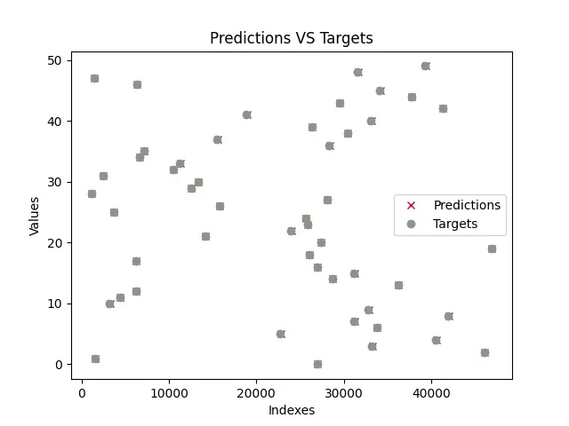
正如我们所看到的,预测几乎与所有真实值重叠(预测由 x 表示,目标由 o 表示)。这意味着该模型几乎成功地预测了 a 和 b 或 m 和 c 的值。
接下来,程序打印在训练模型时发现的所有损失。
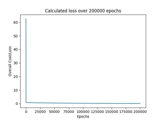
正如我们所看到的,损失立即从 60 左右下降到 0 附近,并在接下来的时期继续保持在附近。
最后,打印训练和测试数据的 RMSE 损失,以及 a 和 b 的预测值或模型参数。
Weights: [0.5008287639956263]
Bias: 1.8339723159878247
RMSE on training data: 0.05855296238504223
RMSE on testing data: 30.609530314187527
我们在这个例子中使用的方程是 y = 0.5x + 2,其中 a = 0.5 和 b = 2。而且,该模型预测了 a = 0.50082 和 b = 1.83397,它们非常接近真实值。这就是为什么我们的预测与真实目标重叠的原因。
在本例中,我们将 epoch 数设置为 200000,将学习率设置为 0.0001。幸运的是,这只是一组给我们带来非常好的、近乎完美的结果的配置。我强烈建议本文的读者尝试使用这些值,看看他们是否可以提出一些可以产生更好结果的值。

Vaibhav is an artificial intelligence and cloud computing stan. He likes to build end-to-end full-stack web and mobile applications. Besides computer science and technology, he loves playing cricket and badminton, going on bike rides, and doodling.