How to Perform Polynomial Regression in R
Polynomial regression can be defined as linear regression in which the relationship between the independent x and dependent y will be modeled as the nth degree polynomial.
This tutorial demonstrates how to perform polynomial regression in R.
Polynomial Regression in R
The polynomial regression will fit a nonlinear relationship between x and the mean of y. It will add the polynomial or quadratic terms to the regression.
This regression is used for one resultant variable and a predictor. The polynomial regression is mainly used in:
- Progression of epidemic diseases
- Calculation of the growth rate of tissues
- Distribution of isotopes of carbon in sediments
We can use ggplot2 to plot the polynomial regression in R. If this package is not yet installed; first, we need to install it:
install.packages('ggplot2')
Here is the step-by-step process of polynomial regression.
Data Creation
We create a data frame with the data of delftstack students: the number of hours studied, final exam marks, and the total number of students in the class, which is 60.
Example:
#create data frame
delftstack <- data.frame(hours = runif(60, 6, 20), marks=60)
delftstack$marks = delftstack$marks + delftstack$hours^3/160 + delftstack$hours*runif(60, 1, 2)

#view the head of the data
head(delftstack)
This code will create the data used later for the polynomial regression.
Output:
      hours     marks
1  7.106636  71.33509
2  8.501039  74.93339
3 18.051042 124.92229
4 19.153316 141.40656
5 18.306620 118.47464
6  6.240467  70.53522
Data Visualization
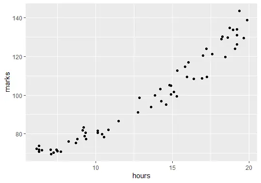
The next step is to visualize the data. Before creating the regression model, we need to show the relationship between the number of hours studied and final exam marks.
Example:
# Visualization
library(ggplot2)

ggplot(delftstack, aes(x=hours, y=marks)) + geom_point()
The code above will plot the graph of our data:
Fit the Polynomial Regression Models
The next step is to fit the polynomial regression models with degrees 1 to 6 and k-fold cross-validation with k=10.
Example:
#shuffle data
delftstack.shuffled <- delftstack[sample(nrow(df)),]

# number of k-fold cross-validation
K <- 10

#define the degree of polynomials to fit
degree <- 6

# now create k equal-sized folds
fold <- cut(seq(1,nrow(delftstack.shuffled)),breaks=K,labels=FALSE)

#The object to hold MSE's of models
mse_object = matrix(data=NA,nrow=K,ncol=degree)

#K-fold cross validation
for(i in 1:K){
    #testing and training data
    test_indexes <- which(fold==i,arr.ind=TRUE)
    test_data <- delftstack.shuffled[test_indexes, ]
    train_data <- delftstack.shuffled[-test_indexes, ]

    # using k-fold cv for models evaluation
    for (j in 1:degree){
        fit.train = lm(marks ~ poly(hours,j), data=train_data)
        fit.test = predict(fit.train, newdata=test_data)
        mse_object[i,j] = mean((fit.test-test_data$marks)^2)
    }
}

# MSE for each degree
colMeans(mse_object)
Output:
[1] 26.13112 15.45428 15.87187 16.88782 18.13103 19.10502
There are six models, and the MSEs for each model are given in the output of the code above. This output is for degrees h=1 to h=6, respectively.
The model with the lowest MSE will be our polynomial regression model, which is h=2 because the MSE value of h=2 is less than all others.
Analyze the Final Model
Finally, let’s analyze the final model and show the summary of the best-fitted model:
Example:
#fitting the best model
best_model = lm(marks ~ poly(hours,2, raw=T), data=delftstack)

#summary of the best model
summary(best_model)
The code above will show the summary of the best-fitted model.
Output:
Call:
lm(formula = marks ~ poly(hours, 2, raw = T), data = delftstack)

Residuals:
   Min     1Q Median     3Q    Max
-8.797 -2.598  0.337  2.443  9.872

Coefficients:
                         Estimate Std. Error t value Pr(>|t|)
(Intercept)              68.42847    5.54533  12.340  < 2e-16 ***
poly(hours, 2, raw = T)1 -1.07557    0.93476  -1.151    0.255
poly(hours, 2, raw = T)2  0.22958    0.03577   6.418 2.95e-08 ***
---
Signif. codes:  0 '***' 0.001 '**' 0.01 '*' 0.05 '.' 0.1 ' ' 1

Residual standard error: 4.204 on 57 degrees of freedom
Multiple R-squared:  0.9669,    Adjusted R-squared:  0.9657
F-statistic: 831.9 on 2 and 57 DF,  p-value: < 2.2e-16
From the output, we can see that marks = 68.42847 - 1.07557*(hours) + .22958*(hours)2. Using this equation, we can predict how many marks a student will get based on the number of hours studied.
For example, if a student studied for 5 hours, the calculation will be:
marks = 68.42847 - 1.07557*(5) + .22958*(5)2

marks = 68.42847 - 1.07557*5 + .22958*25

marks = 68.42847 - 5.37785 + 5.7395

marks = 68.79012
If a student studies for 5 hours, he will get 68.79012 marks in the final exam.
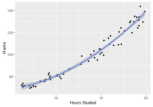
Lastly, we can plot the fitted model to check how well it corresponds to the raw data:
ggplot(delftstack, aes(x=hours, y=marks)) +
    geom_point() +
    stat_smooth(method='lm', formula = y ~ poly(x,2), size = 1) +
    xlab('Hours Studied') +
    ylab('Marks')
Output (Plot):

Sheeraz is a Doctorate fellow in Computer Science at Northwestern Polytechnical University, Xian, China. He has 7 years of Software Development experience in AI, Web, Database, and Desktop technologies. He writes tutorials in Java, PHP, Python, GoLang, R, etc., to help beginners learn the field of Computer Science.
LinkedIn Facebook