How to Perform Logistic Regression in R
The logistic regression is a model in which the response variable has values like True, False, or 0, 1, which are categorical values. It measures the probability of a binary response.
This tutorial will demonstrate how to perform logistic regression in R.
Logistic Regression in R
The glm() method is used in R to create a regression model. It takes three parameters.
First is the formula, which is the symbol that represents the relationship between variables; second is the data which is the data set containing the values of these variables; and third is the family, which is the R object that specifies the details of the model. For logistic regression, the value is binomial.
The mathematical expression for logistic regression is given below:
y = 1/(1+e^-(a+b1x1+b2x2+b3x3+...))
Where:
aandbare the numeric constants which are coefficientsyis the response variablexis the predictor variable
Steps to Perform Logistic Regression in R
Now let’s perform logistic regression in R. Here is the step-by-step process.
Load the Data
Let’s use the default data set from the ISLR package. First, we need to install the package if it is not already installed.
install.packages('ISLR')
Once the package is successfully installed, the next step is to load the data.
require(ISLR)
#load the dataset
data_set <- ISLR::Default

## The total observations in data
nrow(data_set)

#the summary of the dataset
summary(data_set)
The code will load the ISLR default data set and show the number of observations and data summary.
Output:
[1] 10000

 default    student       balance           income
 No :9667   No :7056   Min.   :   0.0   Min.   :  772
 Yes: 333   Yes:2944   1st Qu.: 481.7   1st Qu.:21340
                       Median : 823.6   Median :34553
                       Mean   : 835.4   Mean   :33517
                       3rd Qu.:1166.3   3rd Qu.:43808
                       Max.   :2654.3   Max.   :73554
The data set above contains 10000 individuals.
The default shows whether the individual is defaulted or not, and the student indicates if the individual is a student. The balance means the average balance of an individual, and the income is the individual’s income.
Train and Test Samples
The next step is to split the data set into a training and testing set to train and test the model.
#this will make the example reproducible
set.seed(1)

# We use 70% as training and 30% as testing set
sample <- sample(c(TRUE, FALSE), nrow(data), replace=TRUE, prob=c(0.7,0.3))
train <- data_set[sample, ]
test <- data_set[!sample, ]
Create the Logistic Regression Model
We use glm() to create the logistic regression model with family = binomial.
# the logistic regression model
logistic_model <- glm(default~student+balance+income, family="binomial", data=train)

# just disable scientific notation for summary
options(scipen=999)

# model summary
summary(logistic_model)
The code above creates a logistic regression model and shows the model summary from the data above.
Output:
Deviance Residuals:
    Min       1Q   Median       3Q      Max
-2.4881  -0.1327  -0.0509  -0.0176   3.5912

Coefficients:
                 Estimate    Std. Error z value             Pr(>|z|)
(Intercept) -10.961385538   0.602044982 -18.207 < 0.0000000000000002 ***
studentYes   -0.835485760   0.284855225  -2.933              0.00336 **
balance       0.005893470   0.000289649  20.347 < 0.0000000000000002 ***
income       -0.000001611   0.000009942  -0.162              0.87124
---
Signif. codes:  0 '***' 0.001 '**' 0.01 '*' 0.05 '.' 0.1 ' ' 1

(Dispersion parameter for binomial family taken to be 1)

    Null deviance: 1997.4  on 7014  degrees of freedom
Residual deviance: 1050.9  on 7011  degrees of freedom
AIC: 1058.9

Number of Fisher Scoring iterations: 8
The logistic regression model has been successfully created. Then the next step is to use the model to make predictions.
Use the Model to Make Predictions
Once the logistic regression model is fitted, we can use it to predict if the individual will be in default based on the income, student, or balance status.
#defining two individuals
demo <- data.frame(balance = 1500, income = 3000, student = c("Yes", "No"))

#predict the probability of defaulting
predict(logistic_model, demo, type="response")
The code above predicts the probability of defaulting of two defined individuals.
Output:
         1          2
0.04919576 0.10659389
The probability of an individual defaulting with a balance of $1500, income of $3000, and student status of yes is 0.0491. The same with a student status of no, the probability of default is 0.1065.
Now let’s calculate the probability of defaulting of each individual in our test data set.
#probability of default for the test dataset
prediction <- predict(logistic_model, test, type="response")
The code will calculate the probability of defaulting for each individual in our test data set. The output will be a large sum of data.
The Logistic Regression Model Diagnostics
Now it’s time to check how well our model will perform with the test data set. We find the optimal probability using the optimalCutoff() method from the informationvalue library.
Example:
library(InformationValue)

#from "Yes" and "No" to 1's and 0's
test$default <- ifelse(test$default=="Yes", 1, 0)

#optimal cutoff probability to use for maximize accuracy
optimal <- optimalCutoff(test$default, prediction)[1]
optimal
The optimal probability cutoff to use is given below. Any individual with a higher probability will be considered defaulted.
Output:
[1] 0.5209985
Next, we can use the confusion matrix to show the comparison of our prediction with actual defaults.
Example:
confusionMatrix(test$default, prediction)
Output:
     0  1
0 2868 71
1   10 36
We can also calculate the true positive rate (sensitivity), the true negative rate (specificity), and the misclassification error:
# sensitivity
sensitivity(test$default, prediction)

# specificity
specificity(test$default, prediction)

# total misclassification error rate
misClassError(test$default, prediction, threshold=optimal)
Output:
[1] 0.3364486

[1] 0.9965254

[1] 0.0265
The total misclassification error rate is 2.65% for our model, which means our model can predict outcomes easily because the error rate is very low.
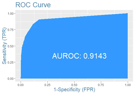
Finally, let’s plot the ROC curve for the test data set with the prediction:
Complete Example Code
Here is the complete code used in this tutorial for your convenience.
install.packages('ISLR')

require(ISLR)
#load the dataset
data_set <- ISLR::Default

## The total observations in data
nrow(data_set)

#the summary of the dataset
summary(data_set)

#this will make the example reproducible
set.seed(1)

#We use 70% of as training set and 30% as testing set
sample <- sample(c(TRUE, FALSE), nrow(data), replace=TRUE, prob=c(0.7,0.3))
train <- data_set[sample, ]
test <- data_set[!sample, ]


# the logistic regression model
logistic_model <- glm(default~student+balance+income, family="binomial", data=train)

# just disable scientific notation for summary
options(scipen=999)

#view model summary
summary(logistic_model)

#defining two individuals
demo <- data.frame(balance = 1500, income = 3000, student = c("Yes", "No"))

#predict the probability of defaulting
predict(logistic_model, demo, type="response")

#probability of default for the test dataset
prediction <- predict(logistic_model, test, type="response")

install.packages('InformationValue')

library(InformationValue)

#from "Yes" and "No" to 1's and 0's
test$default <- ifelse(test$default=="Yes", 1, 0)

#optimal cutoff probability to use for maximize accuracy
optimal <- optimalCutoff(test$default, prediction)[1]
optimal

confusionMatrix(test$default, prediction)

# sensitivity
sensitivity(test$default, prediction)

# specificity
specificity(test$default, prediction)

# total misclassification error rate
misClassError(test$default, prediction, threshold=optimal)

#the ROC curve
plotROC(test$default, prediction)

Sheeraz is a Doctorate fellow in Computer Science at Northwestern Polytechnical University, Xian, China. He has 7 years of Software Development experience in AI, Web, Database, and Desktop technologies. He writes tutorials in Java, PHP, Python, GoLang, R, etc., to help beginners learn the field of Computer Science.
LinkedIn Facebook