R의 로지스틱 회귀
로지스틱 회귀는 응답 변수가 범주 값인 True, False 또는 0, 1과 같은 값을 갖는 모델입니다. 이진 응답의 확률을 측정합니다.
이 튜토리얼은 R에서 로지스틱 회귀를 수행하는 방법을 보여줍니다.
R의 로지스틱 회귀
glm() 메서드는 R에서 회귀 모델을 생성하는 데 사용됩니다. 세 가지 매개변수를 사용합니다.
첫 번째는 변수 간의 관계를 나타내는 기호인 공식입니다. 두 번째는 이러한 변수의 값을 포함하는 데이터 세트인 데이터입니다. 세 번째는 모델의 세부 사항을 지정하는 R 개체인 패밀리입니다. 로지스틱 회귀의 경우 값은 이항입니다.
로지스틱 회귀에 대한 수학적 표현은 다음과 같습니다.
y = 1/(1+e^-(a+b1x1+b2x2+b3x3+...))
어디:
a및b는 계수인 숫자 상수입니다.y는 응답 변수입니다.x는 예측 변수입니다.
R에서 로지스틱 회귀를 수행하는 단계
이제 R에서 로지스틱 회귀를 수행해 보겠습니다. 다음은 단계별 프로세스입니다.
데이터 로드
ISLR 패키지의 기본 데이터 세트를 사용하겠습니다. 먼저 아직 설치되지 않은 경우 패키지를 설치해야 합니다.
install.packages('ISLR')
패키지가 성공적으로 설치되면 다음 단계는 데이터를 로드하는 것입니다.
require(ISLR)
#load the dataset
data_set <- ISLR::Default

## The total observations in data
nrow(data_set)

#the summary of the dataset
summary(data_set)
코드는 ISLR 기본 데이터 세트를 로드하고 관찰 수 및 데이터 요약을 표시합니다.
출력:
[1] 10000

 default    student       balance           income
 No :9667   No :7056   Min.   :   0.0   Min.   :  772
 Yes: 333   Yes:2944   1st Qu.: 481.7   1st Qu.:21340
                       Median : 823.6   Median :34553
                       Mean   : 835.4   Mean   :33517
                       3rd Qu.:1166.3   3rd Qu.:43808
                       Max.   :2654.3   Max.   :73554
위의 데이터 세트에는 10000명의 개인이 포함되어 있습니다.
기본값은 개인의 기본 설정 여부를 나타내고 학생은 개인이 학생인지 여부를 나타냅니다. 잔액은 개인의 평균 잔액을 의미하고 소득은 개인의 소득입니다.
학습 및 테스트 샘플
다음 단계는 데이터 세트를 훈련 및 테스트 세트로 분할하여 모델을 훈련하고 테스트하는 것입니다.
#this will make the example reproducible
set.seed(1)

# We use 70% as training and 30% as testing set
sample <- sample(c(TRUE, FALSE), nrow(data), replace=TRUE, prob=c(0.7,0.3))
train <- data_set[sample, ]
test <- data_set[!sample, ]
로지스틱 회귀 모델 만들기
glm()을 사용하여 family = binomial로 로지스틱 회귀 모델을 만듭니다.
# the logistic regression model
logistic_model <- glm(default~student+balance+income, family="binomial", data=train)

# just disable scientific notation for summary
options(scipen=999)

# model summary
summary(logistic_model)
위의 코드는 로지스틱 회귀 모델을 생성하고 위 데이터의 모델 요약을 보여줍니다.
출력:
Deviance Residuals:
    Min       1Q   Median       3Q      Max
-2.4881  -0.1327  -0.0509  -0.0176   3.5912

Coefficients:
                 Estimate    Std. Error z value             Pr(>|z|)
(Intercept) -10.961385538   0.602044982 -18.207 < 0.0000000000000002 ***
studentYes   -0.835485760   0.284855225  -2.933              0.00336 **
balance       0.005893470   0.000289649  20.347 < 0.0000000000000002 ***
income       -0.000001611   0.000009942  -0.162              0.87124
---
Signif. codes:  0 '***' 0.001 '**' 0.01 '*' 0.05 '.' 0.1 ' ' 1

(Dispersion parameter for binomial family taken to be 1)

    Null deviance: 1997.4  on 7014  degrees of freedom
Residual deviance: 1050.9  on 7011  degrees of freedom
AIC: 1058.9

Number of Fisher Scoring iterations: 8
로지스틱 회귀 모델이 성공적으로 생성되었습니다. 그런 다음 다음 단계는 모델을 사용하여 예측하는 것입니다.
모델을 사용하여 예측하기
로지스틱 회귀 모델이 맞춰지면 이를 사용하여 수입, 학생 또는 균형 상태를 기반으로 개인이 기본에 있는지 여부를 예측할 수 있습니다.
#defining two individuals
demo <- data.frame(balance = 1500, income = 3000, student = c("Yes", "No"))

#predict the probability of defaulting
predict(logistic_model, demo, type="response")
위의 코드는 정의된 두 개인의 불이행 확률을 예측합니다.
출력:
         1          2
0.04919576 0.10659389
잔고 $1500, 소득 $3000, 학생 상태 예로 불이행할 확률은 0.0491입니다. 학생 상태가 아니오인 경우 기본 확률은 0.1065입니다.
이제 테스트 데이터 세트에서 각 개인의 불이행 확률을 계산해 보겠습니다.
#probability of default for the test dataset
prediction <- predict(logistic_model, test, type="response")
이 코드는 테스트 데이터 세트의 각 개인에 대한 불이행 확률을 계산합니다. 출력은 많은 양의 데이터가 됩니다.
로지스틱 회귀 모델 진단
이제 모델이 테스트 데이터 세트로 얼마나 잘 수행되는지 확인할 차례입니다. informationvalue 라이브러리의 optimalCutoff() 메서드를 사용하여 최적의 확률을 찾습니다.
예:
library(InformationValue)

#from "Yes" and "No" to 1's and 0's
test$default <- ifelse(test$default=="Yes", 1, 0)

#optimal cutoff probability to use for maximize accuracy
optimal <- optimalCutoff(test$default, prediction)[1]
optimal
사용할 최적의 확률 컷오프는 다음과 같습니다. 더 높은 확률을 가진 개인은 불이행으로 간주됩니다.
출력:
[1] 0.5209985
다음으로 혼동 행렬을 사용하여 예측과 실제 기본값의 비교를 표시할 수 있습니다.
예:
confusionMatrix(test$default, prediction)
출력:
     0  1
0 2868 71
1   10 36
진양성률(민감도), 진음성률(특이도) 및 오분류 오류도 계산할 수 있습니다.
# sensitivity
sensitivity(test$default, prediction)

# specificity
specificity(test$default, prediction)

# total misclassification error rate
misClassError(test$default, prediction, threshold=optimal)
출력:
[1] 0.3364486

[1] 0.9965254

[1] 0.0265
우리 모델의 총 오분류 오류율은 2.65%입니다. 이는 오류율이 매우 낮기 때문에 모델이 결과를 쉽게 예측할 수 있음을 의미합니다.
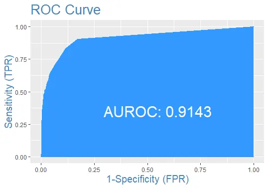
마지막으로 예측이 포함된 테스트 데이터 세트에 대한 ROC 곡선을 플로팅해 보겠습니다.
완전한 예제 코드
다음은 편의를 위해 이 자습서에서 사용된 전체 코드입니다.
install.packages('ISLR')

require(ISLR)
#load the dataset
data_set <- ISLR::Default

## The total observations in data
nrow(data_set)

#the summary of the dataset
summary(data_set)

#this will make the example reproducible
set.seed(1)

#We use 70% of as training set and 30% as testing set
sample <- sample(c(TRUE, FALSE), nrow(data), replace=TRUE, prob=c(0.7,0.3))
train <- data_set[sample, ]
test <- data_set[!sample, ]


# the logistic regression model
logistic_model <- glm(default~student+balance+income, family="binomial", data=train)

# just disable scientific notation for summary
options(scipen=999)

#view model summary
summary(logistic_model)

#defining two individuals
demo <- data.frame(balance = 1500, income = 3000, student = c("Yes", "No"))

#predict the probability of defaulting
predict(logistic_model, demo, type="response")

#probability of default for the test dataset
prediction <- predict(logistic_model, test, type="response")

install.packages('InformationValue')

library(InformationValue)

#from "Yes" and "No" to 1's and 0's
test$default <- ifelse(test$default=="Yes", 1, 0)

#optimal cutoff probability to use for maximize accuracy
optimal <- optimalCutoff(test$default, prediction)[1]
optimal

confusionMatrix(test$default, prediction)

# sensitivity
sensitivity(test$default, prediction)

# specificity
specificity(test$default, prediction)

# total misclassification error rate
misClassError(test$default, prediction, threshold=optimal)

#the ROC curve
plotROC(test$default, prediction)

Sheeraz is a Doctorate fellow in Computer Science at Northwestern Polytechnical University, Xian, China. He has 7 years of Software Development experience in AI, Web, Database, and Desktop technologies. He writes tutorials in Java, PHP, Python, GoLang, R, etc., to help beginners learn the field of Computer Science.
LinkedIn Facebook