R のロジスティック回帰
ロジスティック回帰は、応答変数が True、False、または 0、1 のようなカテゴリ値を持つモデルです。 バイナリ応答の確率を測定します。
このチュートリアルでは、R でロジスティック回帰を実行する方法を示します。
R のロジスティック回帰
glm() メソッドは R で回帰モデルを作成するために使用されます。 3つのパラメーターが必要です。
1つ目は、変数間の関係を表す記号である 式 です。 2 番目は、これらの変数の値を含むデータ セットである data です。 3 番目は、モデルの詳細を指定する R オブジェクトである family です。 ロジスティック回帰の場合、値は二項です。
ロジスティック回帰の数式は次のとおりです。
y = 1/(1+e^-(a+b1x1+b2x2+b3x3+...))
どこ:
aとbは係数である数値定数ですyは応答変数ですxは予測変数です
R でロジスティック回帰を実行する手順
それでは、R でロジスティック回帰を実行してみましょう。これが段階的なプロセスです。
データをロードする
ISLR パッケージのデフォルトのデータ セットを使用してみましょう。 まず、パッケージがまだインストールされていない場合は、パッケージをインストールする必要があります。
install.packages('ISLR')
パッケージが正常にインストールされたら、次のステップはデータをロードすることです。
require(ISLR)
#load the dataset
data_set <- ISLR::Default

## The total observations in data
nrow(data_set)

#the summary of the dataset
summary(data_set)
このコードは、ISLR の既定のデータ セットを読み込み、観測数とデータの概要を表示します。
出力:
[1] 10000

 default    student       balance           income
 No :9667   No :7056   Min.   :   0.0   Min.   :  772
 Yes: 333   Yes:2944   1st Qu.: 481.7   1st Qu.:21340
                       Median : 823.6   Median :34553
                       Mean   : 835.4   Mean   :33517
                       3rd Qu.:1166.3   3rd Qu.:43808
                       Max.   :2654.3   Max.   :73554
上記のデータセットには 10000 人の個人が含まれています。
default は、個人が不履行であるかどうかを示し、student は個人が学生であるかどうかを示します。 balance は個人の平均的な残高を意味し、income は個人の収入です。
サンプルのトレーニングとテスト
次のステップでは、データ セットをトレーニング セットとテスト セットに分割して、モデルのトレーニングとテストを行います。
#this will make the example reproducible
set.seed(1)

# We use 70% as training and 30% as testing set
sample <- sample(c(TRUE, FALSE), nrow(data), replace=TRUE, prob=c(0.7,0.3))
train <- data_set[sample, ]
test <- data_set[!sample, ]
ロジスティック回帰モデルを作成する
glm() を使用して、family = binomial でロジスティック回帰モデルを作成します。
# the logistic regression model
logistic_model <- glm(default~student+balance+income, family="binomial", data=train)

# just disable scientific notation for summary
options(scipen=999)

# model summary
summary(logistic_model)
上記のコードは、ロジスティック回帰モデルを作成し、上記のデータからモデルの概要を表示します。
出力:
Deviance Residuals:
    Min       1Q   Median       3Q      Max
-2.4881  -0.1327  -0.0509  -0.0176   3.5912

Coefficients:
                 Estimate    Std. Error z value             Pr(>|z|)
(Intercept) -10.961385538   0.602044982 -18.207 < 0.0000000000000002 ***
studentYes   -0.835485760   0.284855225  -2.933              0.00336 **
balance       0.005893470   0.000289649  20.347 < 0.0000000000000002 ***
income       -0.000001611   0.000009942  -0.162              0.87124
---
Signif. codes:  0 '***' 0.001 '**' 0.01 '*' 0.05 '.' 0.1 ' ' 1

(Dispersion parameter for binomial family taken to be 1)

    Null deviance: 1997.4  on 7014  degrees of freedom
Residual deviance: 1050.9  on 7011  degrees of freedom
AIC: 1058.9

Number of Fisher Scoring iterations: 8
ロジスティック回帰モデルが正常に作成されました。 次に、モデルを使用して予測を行います。
モデルを使用して予測を行う
ロジスティック回帰モデルが当てはめられると、それを使用して、収入、学生、またはバランスのステータスに基づいて、個人がデフォルトになるかどうかを予測できます。
#defining two individuals
demo <- data.frame(balance = 1500, income = 3000, student = c("Yes", "No"))

#predict the probability of defaulting
predict(logistic_model, demo, type="response")
上記のコードは、定義された 2 人の個人が債務不履行になる確率を予測します。
出力:
         1          2
0.04919576 0.10659389
残高が$1500、収入が$3000、学生ステータスがはいの個人が債務不履行になる確率は0.0491です。 学生ステータスがnoの場合と同様に、デフォルトの確率は0.1065です。
次に、テスト データ セット内の各個人の債務不履行の確率を計算してみましょう。
#probability of default for the test dataset
prediction <- predict(logistic_model, test, type="response")
このコードは、テスト データ セット内の各個人の債務不履行の確率を計算します。 出力は大量のデータになります。
ロジスティック回帰モデルの診断
ここで、モデルがテスト データ セットでどの程度うまく機能するかを確認します。 informationvalue ライブラリの optimalCutoff() メソッドを使用して最適な確率を見つけます。
例:
library(InformationValue)

#from "Yes" and "No" to 1's and 0's
test$default <- ifelse(test$default=="Yes", 1, 0)

#optimal cutoff probability to use for maximize accuracy
optimal <- optimalCutoff(test$default, prediction)[1]
optimal
使用する最適な確率カットオフを以下に示します。 より高い確率を持つ個人は、債務不履行と見なされます。
出力:
[1] 0.5209985
次に、混同行列を使用して、予測と実際のデフォルトの比較を示します。
例:
confusionMatrix(test$default, prediction)
出力:
     0  1
0 2868 71
1   10 36
真陽性率 (感度)、真陰性率 (特異度)、および誤分類誤差も計算できます。
# sensitivity
sensitivity(test$default, prediction)

# specificity
specificity(test$default, prediction)

# total misclassification error rate
misClassError(test$default, prediction, threshold=optimal)
出力:
[1] 0.3364486

[1] 0.9965254

[1] 0.0265
このモデルの合計誤分類エラー率は 2.65% です。これは、エラー率が非常に低いため、モデルが結果を簡単に予測できることを意味します。
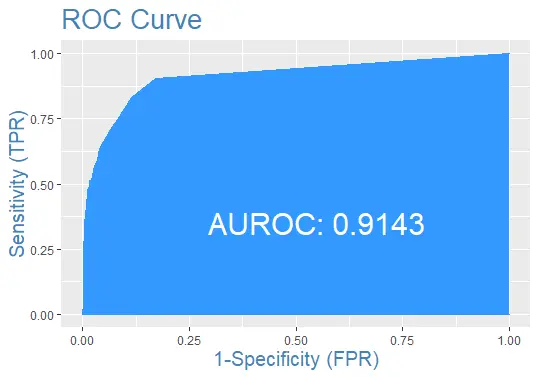
最後に、予測を使用してテスト データ セットの ROC 曲線をプロットしましょう。
完全なサンプルコード
便宜上、このチュートリアルで使用される完全なコードを次に示します。
install.packages('ISLR')

require(ISLR)
#load the dataset
data_set <- ISLR::Default

## The total observations in data
nrow(data_set)

#the summary of the dataset
summary(data_set)

#this will make the example reproducible
set.seed(1)

#We use 70% of as training set and 30% as testing set
sample <- sample(c(TRUE, FALSE), nrow(data), replace=TRUE, prob=c(0.7,0.3))
train <- data_set[sample, ]
test <- data_set[!sample, ]


# the logistic regression model
logistic_model <- glm(default~student+balance+income, family="binomial", data=train)

# just disable scientific notation for summary
options(scipen=999)

#view model summary
summary(logistic_model)

#defining two individuals
demo <- data.frame(balance = 1500, income = 3000, student = c("Yes", "No"))

#predict the probability of defaulting
predict(logistic_model, demo, type="response")

#probability of default for the test dataset
prediction <- predict(logistic_model, test, type="response")

install.packages('InformationValue')

library(InformationValue)

#from "Yes" and "No" to 1's and 0's
test$default <- ifelse(test$default=="Yes", 1, 0)

#optimal cutoff probability to use for maximize accuracy
optimal <- optimalCutoff(test$default, prediction)[1]
optimal

confusionMatrix(test$default, prediction)

# sensitivity
sensitivity(test$default, prediction)

# specificity
specificity(test$default, prediction)

# total misclassification error rate
misClassError(test$default, prediction, threshold=optimal)

#the ROC curve
plotROC(test$default, prediction)

Sheeraz is a Doctorate fellow in Computer Science at Northwestern Polytechnical University, Xian, China. He has 7 years of Software Development experience in AI, Web, Database, and Desktop technologies. He writes tutorials in Java, PHP, Python, GoLang, R, etc., to help beginners learn the field of Computer Science.
LinkedIn Facebook