R の区分的回帰
Sheeraz Gul
2022年8月18日
R
R Regression
区分的回帰は、データに明確なブレークポイントがある場合に使用されます。このチュートリアルでは、R で区分的回帰を実行する方法を示します。
R の区分的回帰
データに明確なブレークポイントがある場合、機能する回帰は区分的回帰になります。区分的回帰は、以下に示すように段階的なプロセスです。
-
データフレームを作成します。
-
データの線形回帰モデルを適合させます。
lm()メソッドを使用してそれを行うことができます。 -
区分的回帰モデルを適合させます。
segmented()メソッドは、segmentedパッケージから使用され、区分的回帰モデルに適合します。 -
plot()メソッドを使用して、最終的な区分的回帰モデルを視覚化します。
次に、上記の手順を使用して例を試してみましょう。例を参照してください:
#Step 1
#create the DataFrame
data<-read.table(text="
Year    Stopped
2015    973
2016    1025
2017    1151
2018    1384
2019    4507
2020    15557
", header=T, sep="")

#first six rows of the data frame
head(data)


#Step2
#fit the simple linear regression model
dput(names(data))
q.lm <- lm(log(Stopped) ~ Year, data)
summary(q.lm)


#Step3
#fit the piecewise regression model to original model,
#estimating a breakpoint at x=14
install.packages('segmented')
library(segmented)

o <- segmented(q.lm, seg.Z = ~Year, psi = 2018)

# view the summary
summary(o)


#Step4
# visulize the piecewise regression model
plot(o)
points(log(Stopped) ~ Year, data)
上記のコードは、さまざまな年に研究を停止した人の区分的回帰モデルを作成します。コードにはいくつかの出力があり、以下に説明します。
ステップ 1 の出力:
  Year Stopped
1 2015     973
2 2016    1025
3 2017    1151
4 2018    1384
5 2019    4507
6 2020   15557
データの先頭を表示します。
ステップ 2 の出力:
Call:
lm(formula = log(Stopped) ~ Year, data = data)

Residuals:
       1        2        3        4        5        6
 0.50759  0.03146 -0.38079 -0.72463 -0.07216  0.63853

Coefficients:
              Estimate Std. Error t value Pr(>|t|)
(Intercept) -1057.9257   279.3081  -3.788   0.0193 *
Year            0.5282     0.1384   3.815   0.0189 *
---
Signif. codes:  0 '***' 0.001 '**' 0.01 '*' 0.05 '.' 0.1 ' ' 1

Residual standard error: 0.5791 on 4 degrees of freedom
Multiple R-squared:  0.7844,	Adjusted R-squared:  0.7305
F-statistic: 14.56 on 1 and 4 DF,  p-value: 0.01886
これは、線形回帰モデルの要約を示しています。
ステップ 3 の出力:
***Regression Model with Segmented Relationship(s)***

Call:
segmented.lm(obj = q.lm, seg.Z = ~Year, psi = 2018)

Estimated Break-Point(s):
              Est. St.Err
psi1.Year 2017.91  0.039

Meaningful coefficients of the linear terms:
              Estimate Std. Error t value Pr(>|t|)
(Intercept) -162.39260   35.56716  -4.566   0.0448 *
Year           0.08400    0.01764   4.761   0.0414 *
U1.Year        1.12577    0.02495  45.121       NA
---
Signif. codes:  0 '***' 0.001 '**' 0.01 '*' 0.05 '.' 0.1 ' ' 1

Residual standard error: 0.02495 on 2 degrees of freedom
Multiple R-Squared: 0.9998,  Adjusted R-squared: 0.9995

Boot restarting based on 6 samples. Last fit:
Convergence attained in 1 iterations (rel. change 3.7909e-16)
これは区分的回帰モデルに適合し、モデルの要約を示します。モデルは 2017.91 年にブレークポイントを検出します。
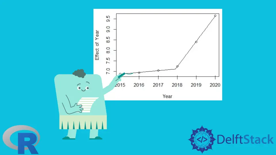
ステップ 4 の出力:

区分的回帰モデルを視覚化します。プロットは、区分的回帰モデルが特定のデータに非常によく適合していることを示しています。
チュートリアルを楽しんでいますか? <a href="https://www.youtube.com/@delftstack/?sub_confirmation=1" style="color: #a94442; font-weight: bold; text-decoration: underline;">DelftStackをチャンネル登録</a> して、高品質な動画ガイドをさらに制作するためのサポートをお願いします。 Subscribe
著者: Sheeraz Gul

Sheeraz is a Doctorate fellow in Computer Science at Northwestern Polytechnical University, Xian, China. He has 7 years of Software Development experience in AI, Web, Database, and Desktop technologies. He writes tutorials in Java, PHP, Python, GoLang, R, etc., to help beginners learn the field of Computer Science.
LinkedIn Facebook