How to Implement Polynomial Regression in Python

1. Definition of Regression
2. Types of Regression
3. Implement Polynomial Regression in Python

This article will light on polynomial regression and how we can apply it to real-world data using Python.

First, we will understand what regression is and how it is different from polynomial regression. Then, we will see the cases where we specifically need polynomial regression.

We will see multiple programming examples alongside to understand the concept better.

Definition of Regression

Regression is a statistical method for determining the relationship between independent variables or characteristics and a dependent variable or result. In machine learning, it is used as a method for predictive modeling, in which an algorithm is employed to anticipate continuous outcomes.

In supervised machine learning, the solution of regression problems is one of the most common applications among machine learning models.

We train the algorithms to find the relationship between a dependent variable and an independent variable to predict some results based on some unseen input data sets.

Regression Models are primarily used in predictive analysis models where applications need to forecast future data based on some input data or historical data. For example, organizations can use regression analysis to predict next month’s sales based on current sales data.

Medical companies can use regression models to forecast health trends in public over a certain period. Typical uses of regression techniques are:

1. Forecasting continuous outcomes, such as property values, stock prices, or sales;
2. Predicting the performance of future retail sales or marketing activities to maximize resource use;
3. Predicting customer or user patterns, such as streaming services or shopping websites;
4. Analyzing datasets to figure out how variables and outputs are related;
5. Predicting interest rates and stock prices based on various factors;
6. Creating visualizations of time series.

Types of Regression

There are many regression techniques, but mainly these are grouped into three main categories:

1. Simple Linear Regression
2. Logistic Regression
3. Multiple Linear Regression

Simple Linear Regression

Simple linear regression is a linear regression approach in which a straight line is plotted within data points to minimize the error between the line and the data points. It’s one of the most fundamental and straightforward forms of machine learning regression.

In this scenario, the independent and dependent variables are considered to have a linear relationship.

Logistic Regression

When the dependent variable can only have two values, true or false, or yes or no, logistic regression is utilized. The chance of a dependent variable occurring can be predicted using logistic regression models.

The output values must, in most cases, be binary. The relationship between the dependent and independent variables can be mapped using a sigmoid curve.

Multiple Linear Regression

Multiple linear regression is used when more than one independent variable is employed. Multiple linear regression techniques include polynomial regression.

When there are many independent variables, it is multiple linear regression. When numerous independent variables are present, it achieves a better fit than basic linear regression.

When displayed in two dimensions, the outcome is a curved line that fits the data points.

In simple regression, we used the following formula to find the value of a dependent variable using an independent value:

$$
y = a+bx+c
$$

Where:

• y is the dependent variable
• a is the y-intercept
• b is the slope
• c is the error rate

In many cases, linear regression will not give the perfect outcome where there is more than one independent variable, for that polynomial regression is needed, which has the formula,

$$
y = a_0 + a_1x_1 + a_2x_2^2 + …..+ a_nx_n^n
$$

As we can see, y is the dependent variable on x.

The degree of this polynomial should have the optimum value as a higher degree overfits the data. With a lower degree value, the model under-fits the results.

Implement Polynomial Regression in Python

Python includes functions for determining a link between data points and drawing a polynomial regression line. Instead of going over the mathematical formula, we’ll show you how to use these strategies.

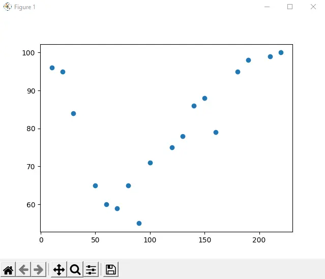
In the example below, 18 automobiles were registered as they passed through a tollbooth. We recorded the car’s speed and the time of day (hour) when it passed us.

The hours of the day are represented on the xAxis, and the speed is represented on the yAxis:

import matplotlib.pyplot as plot

xAxis = [
    10,
    20,
    30,
    50,
    60,
    70,
    80,
    90,
    100,
    120,
    130,
    140,
    150,
    160,
    180,
    190,
    210,
    220,
]
yAxis = [96, 95, 84, 65, 60, 59, 65, 55, 71, 75, 78, 86, 88, 79, 95, 98, 99, 100]

plot.scatter(xAxis, yAxis)
plot.show()

Output:

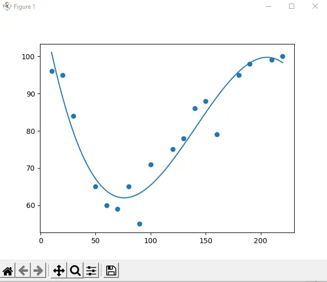
Now, we will draw polynomial regression using NumPy and Matplotlib.

import numpy
import matplotlib.pyplot as plot

xAxis = [
    10,
    20,
    30,
    50,
    60,
    70,
    80,
    90,
    100,
    120,
    130,
    140,
    150,
    160,
    180,
    190,
    210,
    220,
]
yAxis = [96, 95, 84, 65, 60, 59, 65, 55, 71, 75, 78, 86, 88, 79, 95, 98, 99, 100]

model = numpy.poly1d(numpy.polyfit(xAxis, yAxis, 3))

linesp = numpy.linspace(10, 220, 100)

plot.scatter(xAxis, yAxis)
plot.plot(linesp, model(linesp))
plot.show()

Output:

In the above example, we used the libraries NumPy and Matplotlib for drawing polynomial regression by using the import statements. After that, we created arrays for x-axis and y-axis like:

xAxis = [
    10,
    20,
    30,
    50,
    60,
    70,
    80,
    90,
    100,
    120,
    130,
    140,
    150,
    160,
    180,
    190,
    210,
    220,
]
yAxis = [96, 95, 84, 65, 60, 59, 65, 55, 71, 75, 78, 86, 88, 79, 95, 98, 99, 100]

Now, we have used a method of NumPy library for making polynomial model as:

model = numpy.poly1d(numpy.polyfit(xAxis, yAxis, 3))

Now we will specify how to display the line. In our case, we have started it from 10 to 220.

linesp = numpy.linspace(10, 220, 100)

The last three lines of code are used to draw the plot, then the regression line, and then show the plot.

plot.scatter(xAxis, yAxis)
plot.plot(linesp, model(linesp))
plot.show()

The Relationship Between the x-axis and y-axis

It is essential to know the relationship between the axes (x and y) because if there is no relationship between them, it is impossible to predict future values or results from the regression.

We will calculate a value called R-Squared to measure the relationship. It ranges from 0 to 1, where 0 depicts no relationship, and 1 depicts 100% related.

import numpy
import matplotlib.pyplot as plot
from sklearn.metrics import r2_score

xAxis = [
    10,
    20,
    30,
    50,
    60,
    70,
    80,
    90,
    100,
    120,
    130,
    140,
    150,
    160,
    180,
    190,
    210,
    220,
]
yAxis = [96, 95, 84, 65, 60, 59, 65, 55, 71, 75, 78, 86, 88, 79, 95, 98, 99, 100]

model = numpy.poly1d(numpy.polyfit(xAxis, yAxis, 3))

print(r2_score(yAxis, model(xAxis)))

Output:

0.9047652736246418

The value of 0.9 shows the strong relationship between x and y.

If the value is very low, it shows a very weak relationship. Moreover, it indicates that this data set is unsuitable for polynomial regression.