How to Smooth Data in Python

1. Use the Savitzky-Golay Filter to Smooth Data in Python
2. Use the Moving Average to Smooth Data in Python
3. Use the Kernel Regression to Smooth Data in Python
4. Use the Lowess (Locally Weighted Scatterplot Smoothing) to Smooth Data in Python
5. Use the Butterworth Filter to Smooth Data in Python
6. Use the Kalman Filter to Smooth Data in Python
7. Conclusion

Smoothing a curve in a graph is a common preprocessing step in data analysis, enabling clearer visualization of trends while minimizing the impact of noise. In Python, various methods can be employed to achieve this, each with its strengths and applications.

In this article, we will explore several popular smoothing techniques and provide working examples using methods such as Moving Average, Savitzky-Golay Filter, Lowess (Locally Weighted Scatterplot Smoothing), Butterworth Filter, and Kalman Filter.

Use the Savitzky-Golay Filter to Smooth Data in Python

One effective method for dealing with noisy data in a graph is the Savitzky-Golay filter. The Savitzky-Golay filter is a polynomial smoothing filter that works by fitting a polynomial to a local window of data points.

The coefficients of the polynomial are determined using a least-squares approach, providing a smooth output. This method is particularly useful for preserving the shape of the data while reducing noise.

To use the Savitzky-Golay filter in Python, we’ll leverage the savgol_filter function from the scipy.signal module. The syntax is as follows:

smoothed_data = savgol_filter(data, window_size, order)

Parameters:

• data: The input data, typically a 1D array representing the curve to be smoothed.
• window_size: The size of the window used for fitting the polynomial. It should be an odd integer.
• order: The order of the polynomial to be fit. It is recommended to use a small order for gentle smoothing.

Let’s consider a simple example where we have a noisy sine wave that we want to smooth using the Savitzky-Golay filter:

import numpy as np
import matplotlib.pyplot as plt
from scipy.signal import savgol_filter

np.random.seed(42)
x = np.linspace(0, 2 * np.pi, 100)
y_noisy = np.sin(x) + 0.2 * np.random.normal(size=len(x))

window_size = 7
order = 3
y_smoothed = savgol_filter(y_noisy, window_size, order)

plt.figure(figsize=(10, 6))
plt.plot(x, y_noisy, label="Noisy Data", marker="o")
plt.plot(x, y_smoothed, label="Smoothed Data", linestyle="--", linewidth=2)
plt.legend()
plt.title("Smoothing a Curve Using Savitzky-Golay Filter")
plt.xlabel("X-axis")
plt.ylabel("Y-axis")
plt.show()

In the provided example, we first generate a noisy sine wave using numpy and add random noise to simulate real-world data. We then apply the Savitzky-Golay filter to smooth the noisy curve. The window_size and order parameters are tuned based on the characteristics of the data.

The resulting plot illustrates the effectiveness of the Savitzky-Golay filter in reducing noise while preserving the essential features of the underlying curve.

Here, the generated plot displays both the noisy data and the smoothed data, showcasing the impact of the Savitzky-Golay filter on the curve.

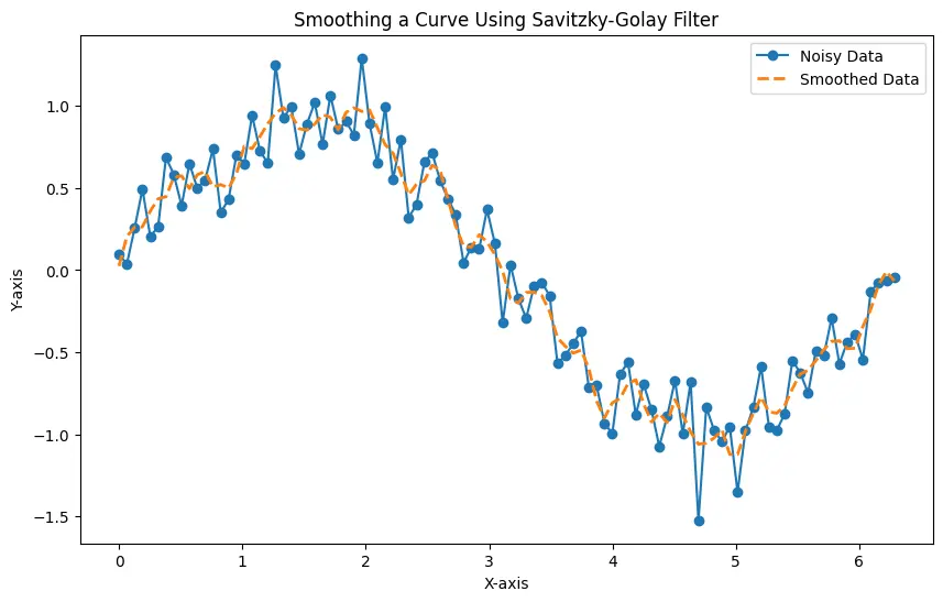
You can adjust the window_size and order parameters based on your specific dataset and requirements. Larger window sizes result in smoother curves, but they might oversmooth the data, removing important details.

Use the Moving Average to Smooth Data in Python

Moving average is another simple yet effective method for smoothing curves in Python. The moving average method involves calculating the average of a set of adjacent data points within a specified window.

This window “moves” along the data, and at each step, the average is computed, producing a smooth curve. This technique is effective in reducing noise and revealing underlying trends.

To apply the moving average in Python, we’ll utilize the rolling function from the pandas library. Here’s the syntax:

smoothed_data = pd.Series(data).rolling(window=window_size, center=True).mean()

Parameters:

• data: The input data, typically a 1D array representing the curve to be smoothed.
• window_size: The size of the window for calculating the moving average. It should be an odd integer for a symmetric window.
• center: A boolean parameter specifying whether the window should be centered around the current data point.

Let’s consider a practical example where we have a noisy sine wave that we want to smooth using a Moving Average:

import numpy as np
import matplotlib.pyplot as plt
import pandas as pd

np.random.seed(42)
x = np.linspace(0, 2 * np.pi, 100)
y_noisy = np.sin(x) + 0.2 * np.random.normal(size=len(x))

window_size = 5
y_smoothed = pd.Series(y_noisy).rolling(window=window_size, center=True).mean()

plt.figure(figsize=(10, 6))
plt.plot(x, y_noisy, label="Noisy Data", marker="o")
plt.plot(x, y_smoothed, label="Smoothed Data", linestyle="--", linewidth=2)
plt.legend()
plt.title("Smoothing a Curve Using Moving Average")
plt.xlabel("X-axis")
plt.ylabel("Y-axis")
plt.show()

Here, we first generate a noisy sine wave using numpy and add random noise to simulate real-world data. We then apply the moving average method to smooth the curve.

The window_size parameter determines the number of adjacent data points used for calculating each average, and setting center=True ensures that the window is symmetrically centered around each data point.

The resulting plot demonstrates the effectiveness of the moving average in reducing noise and providing a clearer representation of the underlying sine wave.

The generated plot displays both the noisy data and the smoothed data, illustrating how the moving average technique can enhance the interpretability of a curve by smoothing out fluctuations.

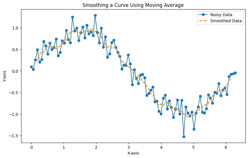
Adjusting the window size allows you to control the level of smoothing, making it a versatile tool for various data analysis tasks.

Use the Kernel Regression to Smooth Data in Python

Kernel Regression is another versatile technique for smoothing curves in Python, offering flexibility in capturing both local and global patterns. Kernel Regression, also known as Nadaraya-Watson regression, involves fitting a kernel (a weighting function) to each data point, and the local weighted average of these kernels is used to predict the value at a given point.

The width of the kernel, controlled by a bandwidth parameter, determines the influence of each neighboring point on the prediction. This technique is effective in capturing both local trends and global patterns in the data.

To apply Kernel Regression in Python, we’ll use the KernelReg class from the statsmodels.nonparametric module. The syntax is as follows:

kernel_regression = sm.nonparametric.KernelReg(
    endog, exog, var_type="c", reg_type="lc", bw="cv_ls"
)
smoothed_data, _ = kernel_regression.fit()

Parameters:

• endog: The dependent variable (the data you want to smooth).
• exog: The independent variable (e.g., the x-values of the curve).
• var_type: Variable type; set to c for continuous.
• reg_type: Regression type; set to lc for locally constant regression.
• bw: Bandwidth; set to cv_ls for automatic bandwidth selection.

Let’s consider a practical example where we have a noisy sine wave that we want to smooth using Kernel Regression:

import numpy as np
import matplotlib.pyplot as plt
import statsmodels.api as sm

np.random.seed(42)
x = np.linspace(0, 2 * np.pi, 100)
y_noisy = np.sin(x) + 0.2 * np.random.normal(size=len(x))

kernel_regression = sm.nonparametric.KernelReg(
    y_noisy, x, var_type="c", reg_type="lc", bw="cv_ls"
)
y_smoothed, _ = kernel_regression.fit()

plt.figure(figsize=(10, 6))
plt.plot(x, y_noisy, label="Noisy Data", marker="o")
plt.plot(x, y_smoothed, label="Smoothed Data", linestyle="--", linewidth=2)
plt.legend()
plt.title("Smoothing a Curve Using Kernel Regression")
plt.xlabel("X-axis")
plt.ylabel("Y-axis")
plt.show()

In this example, we create a noisy sine wave using numpy and then apply Kernel Regression using the KernelReg class from statsmodels. The bandwidth parameter (bw) is set to cv_ls for automatic bandwidth selection based on cross-validation.

The resulting smoothed curve adapts to the local features of the sine wave, effectively reducing noise while preserving the essential shape.

The generated plot displays both the noisy data and the smoothed data, showcasing the effectiveness of Kernel Regression in capturing the underlying structure of the curve while minimizing the impact of noise.

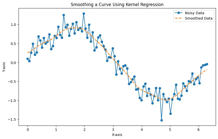
Experimenting with different bandwidth values allows you to fine-tune the smoothing effect based on the characteristics of your data. Note that this method produces a good result but is considered very slow.

Use the Lowess (Locally Weighted Scatterplot Smoothing) to Smooth Data in Python

When it comes to smoothing curves in Python, Lowess or Locally Weighted Scatterplot Smoothing is another valuable tool, especially when dealing with data that exhibits local variations. Lowess is a non-parametric regression technique that fits a smooth curve to data points by locally weighting them.

Unlike global methods, Lowess adapts to the local behavior of the data, making it particularly effective in handling curves with varying slopes and fluctuations. The degree of smoothing is controlled by a parameter called the smoothing fraction.

In Python, the lowess function is available in the statsmodels.api module. Here’s the syntax:

lowess_result = sm.nonparametric.lowess(endog, exog, frac=frac)
smoothed_data = lowess_result[:, 1]

Parameters:

• endog: The dependent variable (the curve to be smoothed).
• exog: The independent variable (e.g., time or position).
• frac: The smoothing fraction, controlling the amount of smoothing. It typically ranges from 0 to 1.

Let’s have an example where we have a noisy sine wave that we want to smooth using Lowess:

import numpy as np
import matplotlib.pyplot as plt
import statsmodels.api as sm

np.random.seed(42)
x = np.linspace(0, 2 * np.pi, 100)
y_noisy = np.sin(x) + 0.2 * np.random.normal(size=len(x))

frac = 0.1
lowess_result = sm.nonparametric.lowess(y_noisy, x, frac=frac)
y_smoothed = lowess_result[:, 1]

plt.figure(figsize=(10, 6))
plt.plot(x, y_noisy, label="Noisy Data", marker="o")
plt.plot(x, y_smoothed, label="Smoothed Data", linestyle="--", linewidth=2)
plt.legend()
plt.title("Smoothing a Curve Using Lowess")
plt.xlabel("X-axis")
plt.ylabel("Y-axis")
plt.show()

In this code example, we first generate a noisy sine wave using numpy and add random noise to simulate real-world data. We then apply Lowess to smooth the curve, setting the smoothing fraction (frac) to 0.1.

The generated plot displays both the noisy data and the smoothed data, illustrating how Lowess effectively captures local trends while reducing the impact of noise.

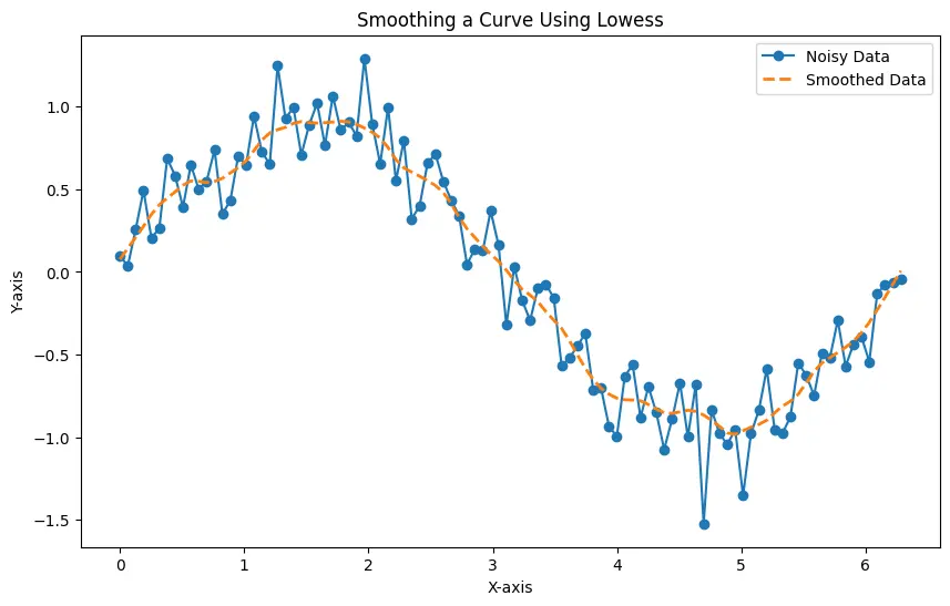
You can adjust the smoothing fraction to control the level of smoothing based on the characteristics of your data, providing flexibility in handling different patterns and noise levels.

Use the Butterworth Filter to Smooth Data in Python

Butterworth filter is also a popular choice for smoothing curves in Python. Its ability to selectively attenuate high-frequency noise while preserving the shape of the signal makes it a valuable tool.

The Butterworth filter is a type of infinite impulse response (IIR) filter that aims to achieve a maximally flat frequency response in the passband. It is commonly used for smoothing time-series data.

The filter has parameters like the cutoff frequency and filter order, which allow users to tailor its behavior to suit specific smoothing requirements.

In Python, the Butterworth filter is implemented through the butter and filtfilt functions in the scipy.signal module. Here’s the syntax:

def butterworth_filter(data, cutoff_freq, sampling_rate, order=4):
    nyquist = 0.5 * sampling_rate
    normal_cutoff = cutoff_freq / nyquist
    b, a = butter(order, normal_cutoff, btype="low", analog=False)
    y_smoothed = filtfilt(b, a, data)
    return y_smoothed

Parameters:

• data: The input data, typically a 1D array representing the curve to be smoothed.
• cutoff_freq: The cutoff frequency separating the passband from the stopband.
• sampling_rate: The sampling rate of the data.
• order: The order of the Butterworth filter, controlling the roll-off.

Suppose we have a noisy sine wave that we want to smooth using the Butterworth filter:

import numpy as np
import matplotlib.pyplot as plt
from scipy.signal import butter, filtfilt


def butterworth_filter(data, cutoff_freq, sampling_rate, order=4):
    nyquist = 0.5 * sampling_rate
    normal_cutoff = cutoff_freq / nyquist
    b, a = butter(order, normal_cutoff, btype="low", analog=False)
    y_smoothed = filtfilt(b, a, data)
    return y_smoothed


np.random.seed(42)
x = np.linspace(0, 2 * np.pi, 100)
y_noisy = np.sin(x) + 0.2 * np.random.normal(size=len(x))

cutoff_freq = 0.1
sampling_rate = 10.0
order = 3
y_smoothed = butterworth_filter(y_noisy, cutoff_freq, sampling_rate, order)

plt.figure(figsize=(10, 6))
plt.plot(x, y_noisy, label="Noisy Data", marker="o")
plt.plot(x, y_smoothed, label="Smoothed Data", linestyle="--", linewidth=2)
plt.legend()
plt.title("Smoothing a Curve Using Butterworth Filter")
plt.xlabel("X-axis")
plt.ylabel("Y-axis")
plt.show()

In this example, we generate the same noisy sine wave and add random noise to simulate real-world data. We then define a function butterworth_filter to apply the Butterworth filter for smoothing.

The parameters, including the cutoff frequency and order, are specified to control the filter’s behavior. The resulting plot illustrates the effectiveness of the Butterworth filter in reducing noise while maintaining the essential features of the sine wave.

The generated plot displays both the noisy data and the smoothed data, showcasing how the Butterworth filter effectively reduces high-frequency noise, providing a clearer representation of the underlying curve.

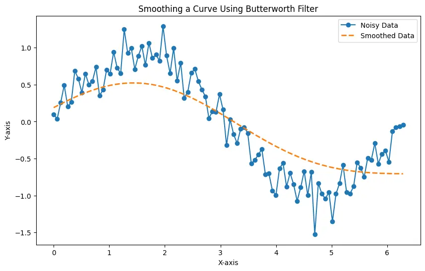
The Butterworth filter is a versatile tool for smoothing curves in Python, offering control over the level of smoothing through parameters like cutoff frequency and order. Experimenting with these parameters allows users to tailor the filter to the specific characteristics of their data, making it a valuable asset in signal processing and data analysis tasks.

Use the Kalman Filter to Smooth Data in Python

The Kalman Filter is another powerful tool for smoothing and estimating states, offering an optimal solution for linear systems with Gaussian noise. It is a recursive algorithm that estimates the state of a dynamic system by combining a prediction of the state with a measurement update.

It is particularly effective in scenarios where the underlying system is linear and subject to Gaussian noise. The Kalman Filter incorporates past measurements and predictions to produce a more accurate and smoothed estimate of the true state of the system.

In Python, the pykalman library provides a convenient implementation of the Kalman Filter. Here’s the syntax:

from pykalman import KalmanFilter


def kalman_filter(data, process_noise=0.1, measurement_noise=0.1):
    kf = KalmanFilter(initial_state_mean=data[0], n_dim_obs=1)
    kf = kf.em(data, n_iter=5)
    (filtered_state_means, _) = kf.filter(data)
    return filtered_state_means

Parameters:

• data: The input time-series data to be smoothed.
• process_noise: The process noise representing the uncertainty in the system dynamics.
• measurement_noise: The measurement noise, representing the uncertainty in the observed data.

Let’s say we have a noisy sine wave that we want to smooth using the Kalman Filter:

import numpy as np
import matplotlib.pyplot as plt
from pykalman import KalmanFilter


def kalman_filter(data, process_noise=0.1, measurement_noise=0.1):
    kf = KalmanFilter(initial_state_mean=data[0], n_dim_obs=1)
    kf = kf.em(data, n_iter=5)
    (filtered_state_means, _) = kf.filter(data)
    return filtered_state_means


np.random.seed(42)
x = np.linspace(0, 2 * np.pi, 100)
y_noisy = np.sin(x) + 0.2 * np.random.normal(size=len(x))

filtered_state_means = kalman_filter(y_noisy)

plt.figure(figsize=(10, 6))
plt.plot(x, y_noisy, label="Noisy Data", marker="o")
plt.plot(x, filtered_state_means, label="Smoothed Data", linestyle="--", linewidth=2)
plt.legend()
plt.title("Smoothing a Curve Using Kalman Filter")
plt.xlabel("X-axis")
plt.ylabel("Y-axis")
plt.show()

In this example, the kalman_filter function is defined to apply the Kalman Filter for smoothing. The Kalman Filter is initialized with the initial state mean, and the em method is used for parameter estimation. Finally, the filter method is applied to obtain the smoothed state means.

The generated plot displays both the noisy data and the smoothed data, showcasing the effectiveness of the Kalman Filter in reducing noise and providing a clear representation of the underlying sine wave.

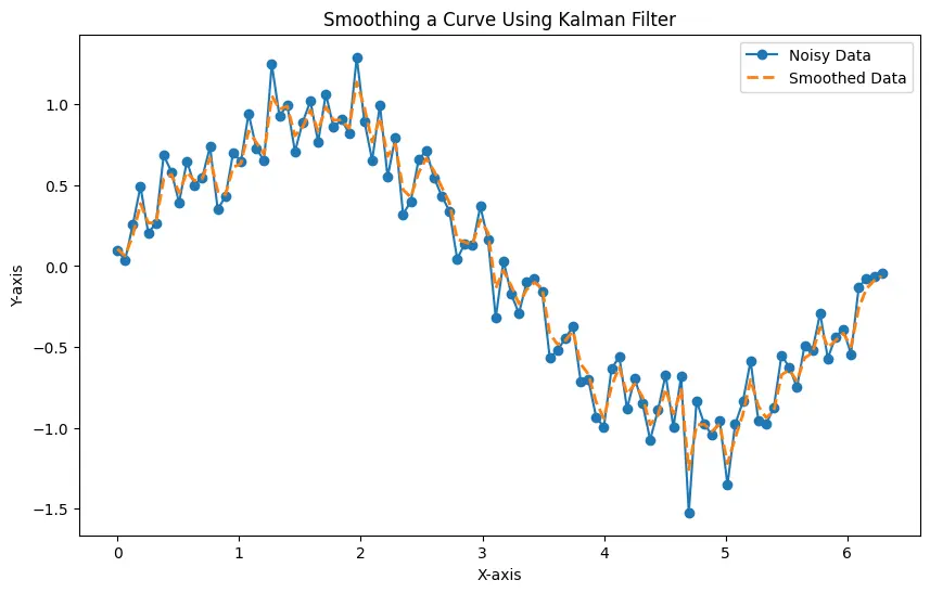
The Kalman Filter is a robust and versatile tool for smoothing time-series data in Python. Its ability to adapt to dynamic systems and handle uncertainties makes it particularly valuable in scenarios where other methods may fall short.

Experimenting with process and measurement noise parameters allows users to tailor the filter to the specific characteristics of their data.

Conclusion

We have explored various powerful methods for smoothing curves in Python, offering a range of techniques suitable for different data characteristics and requirements. Whether you’re dealing with noisy time-series data, preserving local trends, or minimizing high-frequency noise, the presented methods, such as Moving Average, Savitzky-Golay Filter, Lowess, Butterworth Filter, and Kalman Filter, provide versatile solutions.

Experimenting with these techniques empowers data analysts and researchers to enhance visualization and gain clearer insights from their data. Choosing the right smoothing method depends on the specific characteristics of the dataset and the goals of the analysis, allowing for a tailored and effective approach to curve smoothing in Python.