How to Draw Arrow in MATLAB

1. Add Arrows to MATLAB Plots Using the annotation() Function
2. Add Arrows to MATLAB Plots Using the text() Function
3. Add Arrows to MATLAB Plots Using the quiver() Function
4. Conclusion

Adding arrows to plots in MATLAB serves as a valuable technique to enhance visualizations by drawing attention to specific points, emphasizing directional information, or providing additional context to the data. MATLAB offers various methods to incorporate arrows into plots, each with its own set of features and customization options.

Whether utilizing built-in functions like annotation() and text(), or external solutions such as quiver(), mastering arrow addition allows users to create compelling and informative visual representations of their data. This introduction sets the stage for exploring the diverse approaches available in MATLAB for adding arrows to plots, facilitating a deeper understanding of each method’s syntax, functionality, and practical applications.

Add Arrows to MATLAB Plots Using the annotation() Function

Adding arrows to plots in MATLAB can be achieved effortlessly using the versatile annotation() function.

The annotation() function in MATLAB is a versatile tool for adding annotations to figures. It supports various annotation types, including arrows.

By using this function, users can precisely position and customize arrows on their plots.

The basic syntax for adding an arrow using the annotation() function is as follows:

annotation('arrow', [x_start, x_end], [y_start, y_end]);

Here, [x_start, x_end] and [y_start, y_end] represent the x and y coordinates of the starting and ending points of the arrow, respectively.

Code Example 1: Basic Arrow Addition

Let’s consider a simple example where we have a plot, and we want to add an arrow pointing to a specific data point. Assume we have the following data:

% Creating a simple plot
x = 1:0.1:5;
y = sin(x);
plot(x, y, 'LineWidth', 2);

% Adding a basic arrow using annotation()
arrowStart = [0.2, 0.5];
arrowEnd = [0.2, 0.6];
annotation('arrow', arrowStart, arrowEnd, 'LineWidth', 2);

In this example, we begin by creating a simple plot of a sine wave using the plot function. Once the plot is established, we proceed to add a basic arrow using the annotation() function.

The variables arrowStart and arrowEnd are defined to specify the arrow’s starting and ending positions (x, y). The annotation('arrow', arrowStart, arrowEnd, 'LineWidth', 2); call then incorporates the arrow into the plot.

This straightforward example serves as a foundation for understanding the basic application of the annotation() function to add arrows to MATLAB plots.

Output:

Code Example 2: Customizing Arrow Properties

The annotation() function allows users to customize arrows further by specifying additional properties. Here’s an example with some customization:

% Creating another plot
theta = linspace(0, 2*pi, 100);
radius = 2;
x = radius * cos(theta);
y = radius * sin(theta);

figure;
plot(x, y, 'r', 'LineWidth', 2);

% Customizing arrow properties
arrowStart = [0.2, 0.5]; % Starting point of the arrow
arrowEnd = [0.1, 0.5]; % Length and direction of the arrow

arrowHandle = annotation('arrow', arrowStart, arrowEnd);
arrowHandle.Color = [0.1, 0.8, 0.2];
arrowHandle.LineWidth = 3;
arrowHandle.HeadStyle = 'cback2';

In this example, we create a circular plot using the plot function, forming a visually interesting shape. Subsequently, we delve into customizing the properties of the arrow that we add to the plot.

The arrowStart and arrowEnd variables still dictate the arrow’s position and dimensions, but now we introduce a arrowHandle variable. This handle allows us to access and modify the properties of the arrow dynamically after its creation.

The arrow’s color, line width, and head style are customized to demonstrate the flexibility offered by the annotation() function.

Output:

Add Arrows to MATLAB Plots Using the text() Function

In addition to the annotation() function, MATLAB offers another powerful tool for adding arrows to plots— the text() function. While the annotation() function provides a straightforward way to draw arrows with specified properties, the text() function allows for even more flexibility and customization.

The text() function in MATLAB is primarily used for adding text annotations to plots. However, by taking advantage of Unicode characters, it is possible to create arrows dynamically.

The basic syntax for adding an arrow using the text() function is as follows:

text(x, y, '→', 'FontSize', fontSize, 'Color', arrowColor);

Here, (x, y) represents the coordinates of the arrow’s starting point, and the arrow symbol '→' is used to depict the arrowhead. You can customize properties such as font size and color to tailor the appearance of the arrow.

Code Example 1: Basic Arrow Addition Using text()

% Generating a simple plot
t = 1:0.1:5;
plot(t, sin(t), 'LineWidth', 2);

% Adding an arrow using the text() function
arrowX = 2.7;
arrowY = 0.5;
text(arrowX, arrowY, '\leftarrow Basic Arrow');

In this initial example, we begin by generating a plot of a sine wave. After creating the plot, the text() function is employed to add a basic arrow at specific coordinates (arrowX and arrowY).

The text string \leftarrow Basic Arrow includes a left-pointing arrow along with descriptive text. This simple illustration highlights the straightforward use of the text() function to introduce arrows to MATLAB plots.

Output:

Code Example 2: Customizing Arrow Properties With text()

% Creating another plot
theta = linspace(0, 2*pi, 100);
radius = 2;
x = radius * cos(theta);
y = radius * sin(theta);

figure;
plot(x, y, 'r', 'LineWidth', 2);

% Customizing arrow properties
arrowX = 1.5;
arrowY = 1.5;
text(arrowX, arrowY, '\leftarrow Customized Arrow', 'Color', [0.1, 0.8, 0.2], 'FontSize', 12);

In this example, a plot of a circular shape is generated, and the text() function is used to add an arrow at specific coordinates. The arrow is customized by setting its color to a greenish hue and adjusting the font size.

The text() function’s versatility allows users to not only add arrows but also customize their appearance, providing a visually appealing and informative plot.

Output:

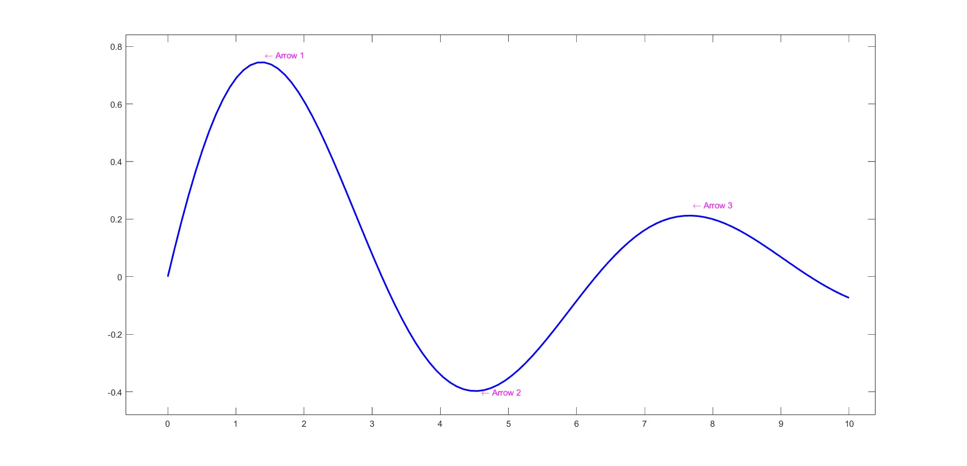
Code Example 3: Multiple Arrows With Dynamic Text Using text()

% Generating a third plot
x = linspace(0, 10, 100);
y = exp(-0.2*x) .* sin(x);

figure;
plot(x, y, 'b', 'LineWidth', 2);

% Adding multiple arrows with dynamic text
arrows = [1.42, 0.77; 4.6, -0.4; 7.7, 0.25];
for i = 1:size(arrows, 1)
    arrowX = arrows(i, 1);
    arrowY = arrows(i, 2);
    text(arrowX, arrowY, sprintf('\\leftarrow Arrow %d', i), 'Color', 'm', 'FontSize', 10);
end

The above example demonstrates the capability of the text() function to add multiple arrows with dynamic text labels. A plot featuring an exponentially decaying sine function is created, and a loop is employed to iterate through the rows of the arrows matrix, allowing for the creation of distinct arrows at different positions on the plot.

The dynamic text labels include both an arrow symbol and a numerical identifier, showcasing the flexibility of the text() function for creating informative and dynamic annotations.

Output:

These examples showcase the flexibility of the text() function for adding arrows to MATLAB plots. By understanding the syntax and exploring customization options, users can enhance their visualizations with informative annotations. The ability to dynamically generate arrows and customize their properties offers a powerful tool for creating compelling and explanatory plots.

Add Arrows to MATLAB Plots Using the quiver() Function

While the annotation() and text() functions are versatile tools for adding arrows to MATLAB plots, another dedicated function exists for precisely this purpose—the quiver() function.

The quiver() function is specifically designed for visualizing vector fields, making it an excellent choice for adding arrows to represent directional information in your plots. It is commonly used in fields such as physics, engineering, and data visualization to depict vector fields.

The quiver() function in MATLAB is designed to create 2D vector plots. Its syntax involves specifying the starting points, lengths, and directions of arrows, allowing for a wide range of customization.

The basic syntax is as follows:

quiver(X, Y, U, V)

Here, X and Y represent the grid coordinates of the arrow starting points, while U and V denote the arrow lengths and directions. Additional parameters can be adjusted to customize the appearance of arrows.

Let’s walk through a few examples of how to use the quiver() function to add arrows to a plot:

Code Example 1: Basic Arrow Plot

% Generating a simple plot
x = linspace(-pi, pi, 20);
y = sin(x);

figure;
plot(x, y, 'LineWidth', 2);
hold on; % To keep the existing plot and add arrows

% Adding arrows using the quiver() function
arrowX = x(1:2:end);
arrowY = y(1:2:end);
arrowU = cos(x(1:2:end));
arrowV = sin(x(1:2:end));

quiver(arrowX, arrowY, arrowU, arrowV, 0, 'color', 'blue', 'MaxHeadSize', 0.1);

title('Sinusoidal Function');
xlabel('X-axis');
ylabel('Y-axis');
grid on;
legend('sin(x)', 'Arrows');
hold off; % Release the hold on the plot

In our first example, we begin by creating a simple plot of a sine wave. To add arrows to the plot, we utilize the quiver() function.

The starting points of the arrows (arrowX and arrowY) are selected at regular intervals along the sine curve. The lengths and directions of the arrows (arrowU and arrowV) are determined by the cosine and sine values, respectively.

The arrows are displayed in blue, and the MaxHeadSize property is set to 0.1 to control the size of the arrowheads. This basic arrow plot demonstrates how the quiver() function can be used to visualize directional information on a curve.

Output:

Code Example 2: Customizing Arrow Properties

% Creating another plot
theta = linspace(0, 2*pi, 20);
r = 1 + sin(3*theta);
[x, y] = pol2cart(theta, r);

figure;
plot(x, y, 'r', 'LineWidth', 2);
hold on;

% Customizing arrow properties using quiver()
quiverX = x(1:2:end);
quiverY = y(1:2:end);
quiverU = cos(theta(1:2:end));
quiverV = sin(theta(1:2:end));

quiver(quiverX, quiverY, quiverU, quiverV, 'color', [0.1, 0.8, 0.2], 'LineWidth', 1.5, 'MaxHeadSize', 0.8);

% Customize plot appearance
title('Polar Plot with Arrows');
xlabel('X-axis');
ylabel('Y-axis');
grid on;
legend('r = 1 + sin(3\theta)', 'Arrows');
axis equal; % Ensure equal scaling for x and y axes
hold off;

In our second example, we generate a polar plot and enhance it by adding arrows using the quiver() function. The starting points of the arrows (quiverX and quiverY) are selected based on polar coordinates.

The lengths and directions of the arrows (quiverU and quiverV) are determined by the cosine and sine values of the polar angles. The arrows are customized by setting the color to a greenish hue, adjusting the line width to 1.5, and controlling the maximum head size.

This example illustrates the versatility of the quiver() function for adding arrows to different types of plots.

Output:

Conclusion

Adding arrows to plots in MATLAB can be accomplished through various methods, each offering unique features and customization options. The choice of method depends on the specific requirements of the visualization.

The built-in annotation() function allows the creation of arrows using precise coordinates and offers extensive customization options such as color, line style, and head style. It is especially useful for straightforward arrow additions to existing plots.

Another built-in function, text(), is versatile for adding arrows by specifying coordinates and utilizing text annotations. This method is suitable for users who prefer a straightforward approach and want to incorporate arrows with customized text labels.

The quiver() function is designed for creating 2D vector plots and is effective for visualizing vector fields or directional information. It offers flexibility in specifying arrow starting points, lengths, and directions, making it suitable for applications involving vector fields.

MATLAB provides multiple avenues to enhance plots with arrows, catering to diverse needs. You can choose the method that aligns with your preferences, the complexity of the visualization, and the level of customization required.

Whether it’s the built-in functions like annotation() and text(), or external options like quiver() and arrow(), MATLAB provides a robust set of tools for creating informative and visually appealing plots.