How to Plot Exponential Function of Any Equation in MATLAB

1. Plot Exponential Functions in MATLAB With the plot Function
2. Customize Exponential Function Plot in MATLAB With the plot Function
3. Plot Exponential Functions in MATLAB With the semilogy Function
4. Plot Multiple Exponential Functions on the Same Plot in MATLAB
5. Conclusion

Exponential functions are fundamental in various scientific and engineering disciplines, representing phenomena characterized by rapid growth or decay. MATLAB, a versatile numerical computing environment, provides an array of tools for plotting and analyzing these functions.

This article serves as a guide on how to plot an exponential function of any equation under observation in MATLAB, offering insights into different approaches and customization options. Whether you are exploring the behavior of a specific exponential model or comparing multiple functions, MATLAB empowers you to create informative and visually appealing plots.

Plot Exponential Functions in MATLAB With the plot Function

MATLAB, with its powerful plotting capabilities, offers a straightforward approach to visualize these functions using the plot function.

The plot function is a fundamental tool for creating 2D plots. It takes two input vectors, x and y, and connects the points defined by these vectors with lines.

The basic syntax of the plot function is as follows:

plot(X, Y)

• X: Vector of x-coordinates. This could be a numeric vector or a time series.
• Y: Vector of y-coordinates corresponding to the x-coordinates in X.

For plotting exponential functions, we first define a range of x values using the linspace function. Then, we calculate the corresponding y values using the exponential function exp(x).

Finally, we use the plot function to visualize the exponential function on a Cartesian plane.

Code Example:

% Define the exponential function
x = linspace(0, 5, 100); % Create a range of x values
y = exp(x); % Exponential function

% Plot the exponential function
figure;
plot(x, y, 'LineWidth', 2);
title('Basic Exponential Function Plot');
xlabel('x');
ylabel('y');
grid on;

In this code example, we start by defining a range of x values using the linspace function, spanning from 0 to 5 with 100 points. The exponential function exp(x) is then applied to generate the corresponding y values.

The plot function is employed to create a simple 2D plot, where x represents the x-axis values, y represents the y-axis values, and the option 'LineWidth', 2 sets the thickness of the plot line.

The title, xlabel, and ylabel functions add a title and labels to the plot for better clarity. Lastly, grid on adds a grid to enhance readability.

This basic approach is ideal for quickly visualizing the shape and behavior of an exponential function.

Code Output:

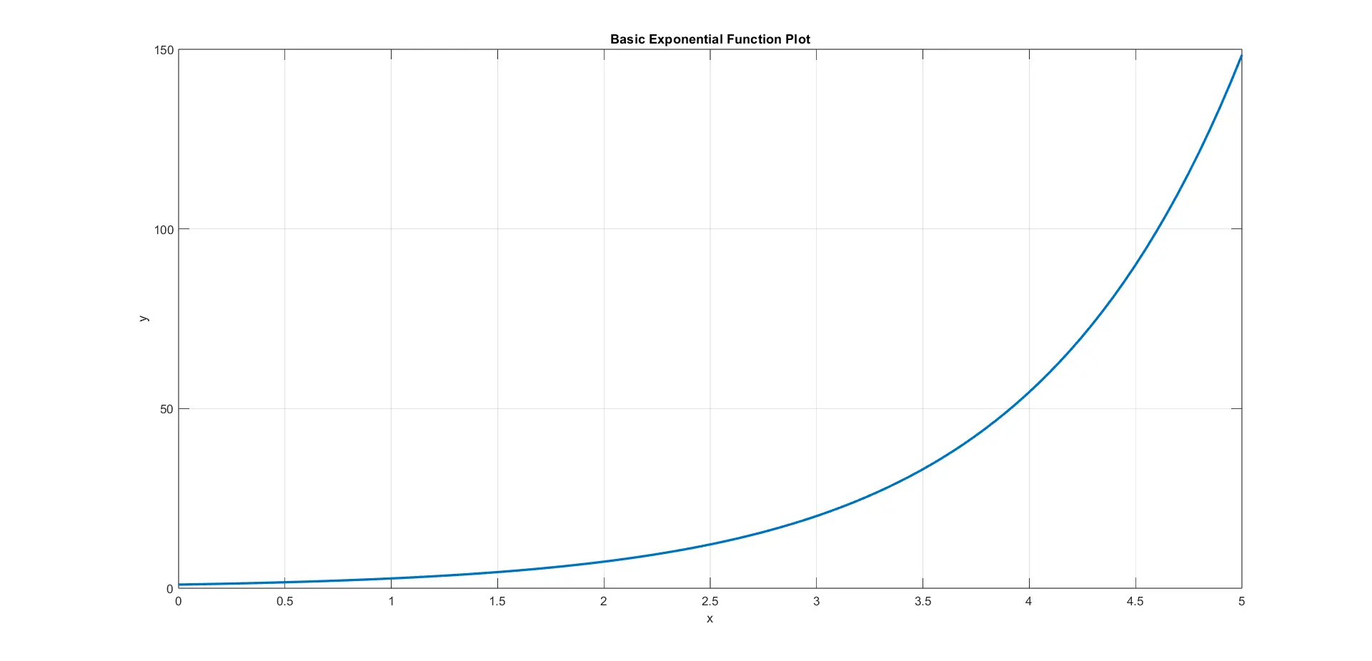
The output of this code is a clean and straightforward 2D plot of the exponential function, clearly showing the exponential growth as x increases. The plotted curve also has a smooth and continuous appearance, demonstrating the characteristic behavior of an exponential function.

Customize Exponential Function Plot in MATLAB With the plot Function

You can also customize the appearance of the plot by including additional formatting options after the X, Y pairs. For example:

plot(X, Y, 'LineStyle', '--', 'Color', 'red', 'Marker', 'o', 'LineWidth', 2)

Here:

• 'LineStyle', '--': This sets the line style to dashed.
• 'Color', 'red': This sets the line color to red.
• 'Marker', 'o': This adds circular markers along the line.
• 'LineWidth', 2: This sets the line width to 2 points.

In the example below, we take the basic exponential function plot and customize its appearance. We use the plot function, but this time, we introduce additional parameters to control the line style, color, and markers.

This enables us to create visually distinct plots, making it easier to differentiate between various functions or highlight specific characteristics.

Code Example:

% Define the exponential function
x = linspace(0, 5, 100);
y = exp(x);

% Customize the plot appearance
figure;
plot(x, y, 'r--o', 'LineWidth', 2, 'MarkerSize', 8);
title('Customized Exponential Function Plot');
xlabel('x');
ylabel('y');
grid on;

In this code example, we use the plot function with additional parameters: 'r--o'. Here, 'r' specifies the color red, '--' denotes a dashed line, and 'o' represents circular markers.

Similar to the previous example, we set the title, xlabel, and ylabel to add context to the plot. The grid on command is included to enhance the readability of the plot.

By adjusting these parameters, you can create customized plots that cater to specific preferences or align with the requirements of your analysis. This flexibility is particularly useful when dealing with multiple functions on the same plot or when emphasizing particular features of the data.

Code Output:

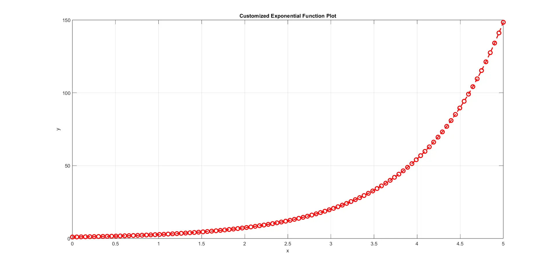
As you can see, a new figure window appears, showcasing a visually customized plot of the exponential function. The red dashed line with circular markers provides a distinctive appearance, making the plot more engaging and facilitating a clearer interpretation of the underlying data.

This level of customization is valuable when presenting results or findings in a visually appealing manner.

Plot Exponential Functions in MATLAB With the semilogy Function

In this approach, we use the semilogy function in MATLAB, which creates plots with logarithmic scaling on the y-axis. The basic syntax of the semilogy function is as follows:

semilogy(X, Y)

• X: Vector of x-coordinates.
• Y: Vector of y-coordinates corresponding to the x-coordinates in X.

This function works similarly to the plot function, but it applies a logarithmic scale to the y-axis. The semilogy function can also take additional formatting options for customization.

For example, you can include a line style, color, and marker as follows:

semilogy(X, Y, 'LineStyle', '--', 'Color', 'red', 'Marker', 'o', 'LineWidth', 2)

Where:

• 'LineStyle', '--': This sets the line style to dashed.
• 'Color', 'red': This sets the line color to red.
• 'Marker', 'o': This adds circular markers along the line.
• 'LineWidth', 2: This sets the line width to 2 points.

These additional options allow you to customize the appearance of the plot created with semilogy in a similar fashion to the plot function.

By applying a logarithmic scale to the y-axis, we can better visualize exponential growth, as the characteristic curve of exponential functions often appears as a straight line on a logarithmic scale. This technique is particularly beneficial when dealing with data that spans several orders of magnitude.

Code Example:

% Define the exponential function
x = linspace(0, 5, 100);
y = exp(x);

% Plot on logarithmic axes
figure;
semilogy(x, y, 'b', 'LineWidth', 2);
title('Exponential Function on Logarithmic Axes');
xlabel('x');
ylabel('y');
grid on;

In the MATLAB code example above, the semilogy function is a key component, offering the ability to plot data on a logarithmic scale along the y-axis. This is particularly valuable when dealing with exponential growth or decay, as the characteristic curve of such functions often manifests as a straight line on a logarithmic scale.

In the code, we define a range of x values using the linspace function and calculate the corresponding y values using the exponential function exp(x). By invoking the semilogy function with the specified line properties in blue and a line width of 2, we create a plot that effectively captures the exponential behavior on logarithmic axes.

The title, xlabel, and ylabel are set to provide context to the plot, while the grid on command enhances the readability of the logarithmic representation.

Code Output:

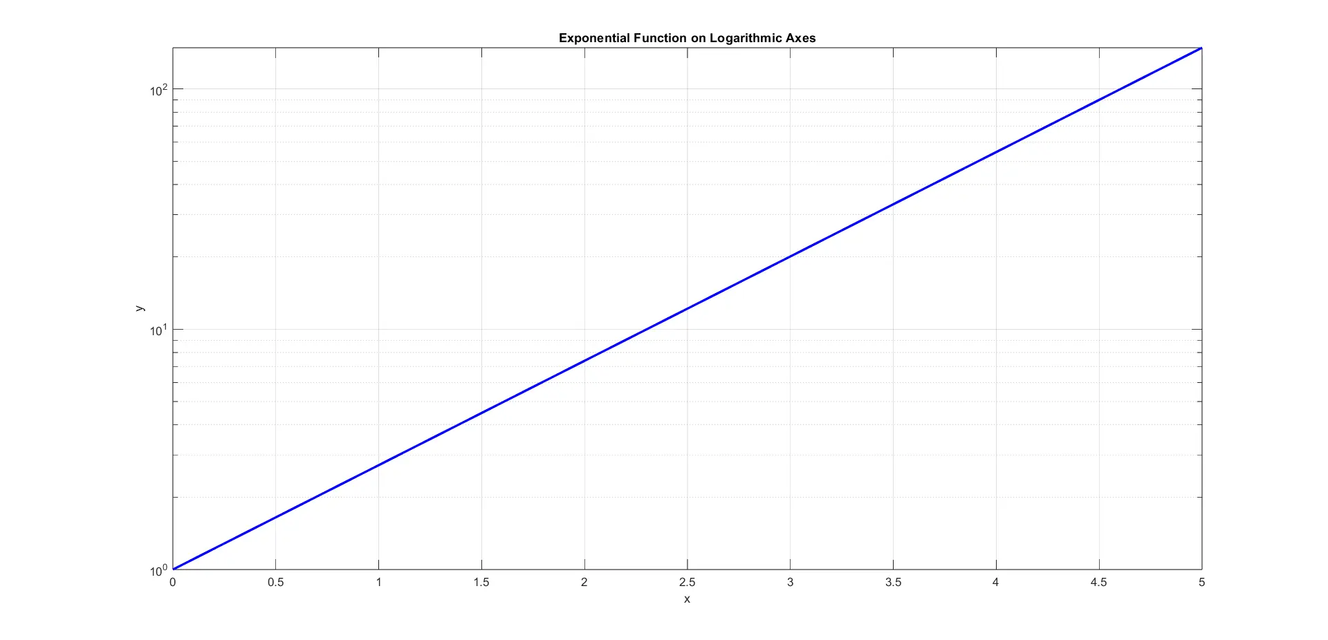
As you can see, a new figure window appears, displaying the exponential function plotted on logarithmic y-axes. The resulting plot reveals a straight line, emphasizing the exponential nature of the function.

This logarithmic representation provides a valuable perspective, making it easier to analyze and interpret the exponential behavior within the given range of x values.

Plot Multiple Exponential Functions on the Same Plot in MATLAB

To plot multiple exponential functions on the same graph, we can employ the plot function with multiple pairs of x and y vectors. Each pair represents a distinct exponential function.

By using the hold on and hold off commands, we can overlay these functions on the same plot without clearing the existing figure. Additionally, the legend function helps differentiate between the functions by providing labels for each.

Code Example:

% Define multiple exponential functions
x = linspace(0, 5, 100);
y1 = exp(x);
y2 = 2 * exp(x);
y3 = 0.5 * exp(x);

% Plot multiple exponential functions
figure;
plot(x, y1, 'LineWidth', 2, 'DisplayName', 'exp(x)');
hold on;
plot(x, y2, 'LineStyle', '--', 'LineWidth', 2, 'DisplayName', '2 * exp(x)');
plot(x, y3, 'LineStyle', '-.', 'LineWidth', 2, 'DisplayName', '0.5 * exp(x)');
hold off;

title('Multiple Exponential Functions Plot');
xlabel('x');
ylabel('y');
legend('show');
grid on;

In this code example, we define three sets of y values (y1, y2, and y3), each corresponding to a different exponential function.

The plot function is used to plot each exponential function with specified line properties. The hold on command ensures that subsequent plots overlay the existing figure, and hold off terminates the overlay.

The legend function provides labels for each function.

Standard properties such as title, xlabel, and ylabel are set to add context to the plot. The grid on command adds a grid for better readability.

By utilizing this approach, we can visually compare and contrast multiple exponential functions, aiding in the analysis of their growth or decay patterns within the specified x range.

Code Output:

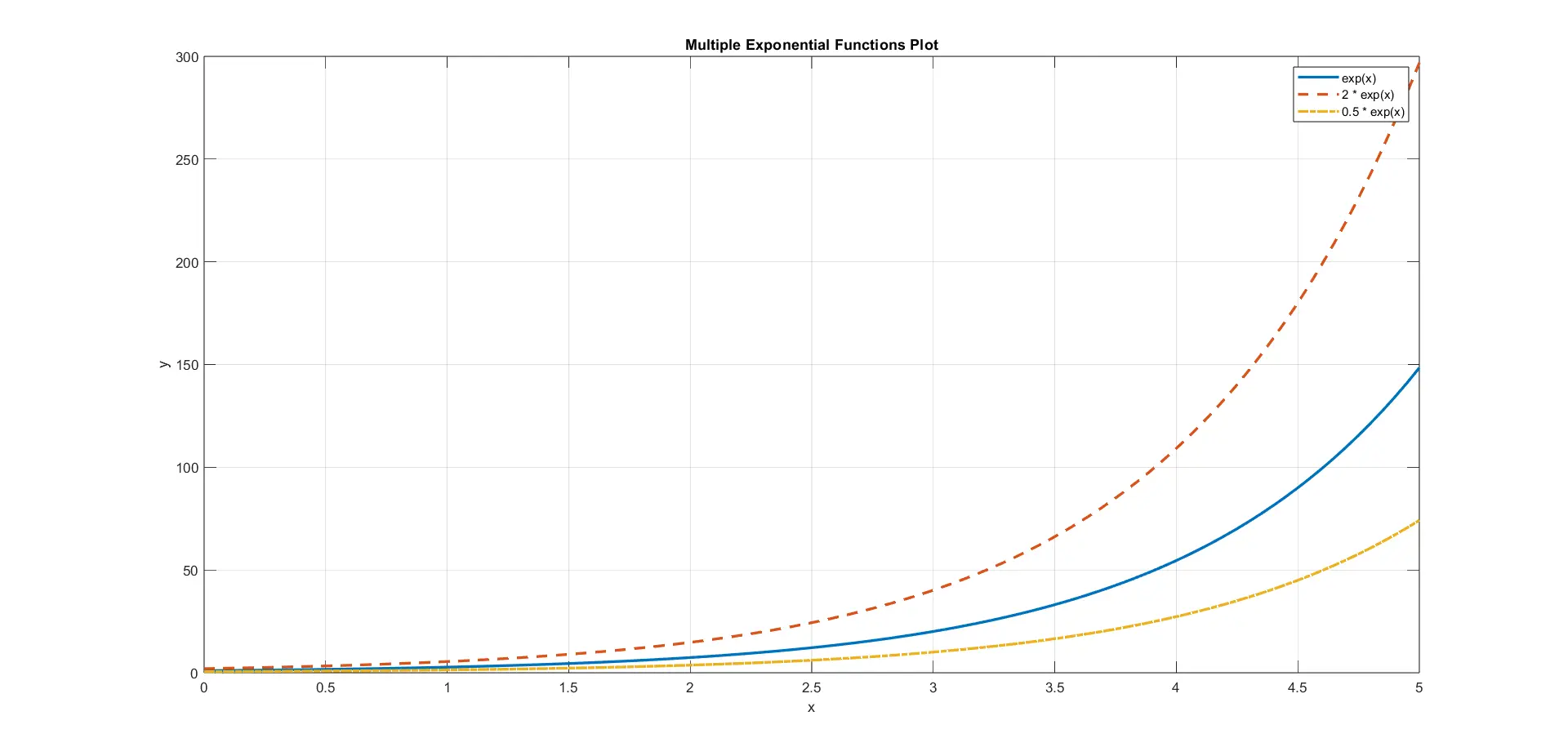
Upon execution, the code produces a figure with three exponential functions plotted on the same graph. The legend clearly identifies each function, and the distinctive line styles and colors help differentiate their behavior.

Conclusion

MATLAB stands out as a powerful ally for researchers, engineers, and scientists seeking to visualize and analyze exponential functions. The flexibility of MATLAB’s plotting functions, combined with the ability to customize appearance and compare multiple functions on the same graph, enables a comprehensive exploration of exponential behavior.

Whether you are studying biological growth, financial trends, or physical decay, MATLAB’s intuitive plotting capabilities provide a valuable tool for gaining insights and making informed decisions based on your observations.