How to Create a 3D Plot Using Seaborn and Matplotlib

In this explanation, we look at what a 3D plot is, and we also learn how we can create several different 3D plots With the help of seaborn and matplotlib.
Create a 3D Plot Using Seaborn and Matplotlib
Let’s get started by importing Matplotlib, NumPy, and Seaborn.
import seaborn as seaborn
import matplotlib.pyplot as plot
import numpy as np
Now we are using NumPy’s random module to create some x, y, and z data, and we have a total of 50 points.
mean = 3
number = 50

x1 = np.random.normal(mean, 1, size=number)
y1 = np.random.normal(mean, 1, size=number)
z1 = np.random.normal(mean, 1, size=number)
There are several different 3D plots we can make with Matplotlib. Whenever we want to plot in 3D with Matplotlib, we will first need to start by creating a set of axes using the axes() function.
We will use the projection keyword and pass the 3D value as a string. This will tell Matplotlib that we will create something in three dimensions.
plot.figure(figsize=(6, 5))
axes = plot.axes(projection="3d")
If we check the type of axes, we will see that these are 3D subplot axes.
print(type(axes))
Output:
<class 'matplotlib.axes._subplots.Axes3DSubplot'>
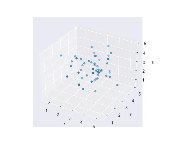
We will need to call the scatter3D() function and pass our x, y, and z data points. This isn’t easy to represent which one is the x-axis, y-axis, etc., so let’s set the labels for the 3 dimensions.
import seaborn as seaborn
import matplotlib.pyplot as plot
import numpy as np

seaborn.set_style("darkgrid")

mean = 3
number = 50

x1 = np.random.normal(mean, 1, size=number)
y1 = np.random.normal(mean, 1, size=number)
z1 = np.random.normal(mean, 1, size=number)

plot.figure(figsize=(6, 5))
axes = plot.axes(projection="3d")
print(type(axes))
axes.scatter3D(x1, y1, z1)

axes.set_xlabel("x")
axes.set_ylabel("y")
axes.set_zlabel("z")
plot.show()
Output:
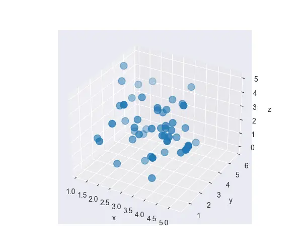
If we want to increase the scatter points’ size, we can reference this s argument and increase that to 100.
import seaborn as seaborn
import matplotlib.pyplot as plot
import numpy as np

seaborn.set_style("darkgrid")

mean = 3
number = 50

x1 = np.random.normal(mean, 1, size=number)
y1 = np.random.normal(mean, 1, size=number)
z1 = np.random.normal(mean, 1, size=number)

plot.figure(figsize=(6, 5))
axes = plot.axes(projection="3d")
print(type(axes))
axes.scatter3D(x1, y1, z1, s=100)

axes.set_xlabel("x")
axes.set_ylabel("y")
axes.set_zlabel("z")
plot.show()
Output:
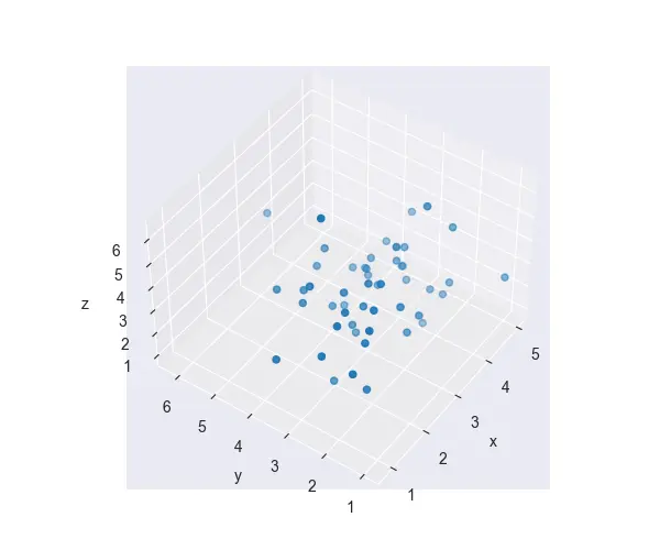
We can rotate this three-dimensional figure using the view_init() method. This method accepts two arguments, the first will be the angle of our elevation, and the second one will be the angle of our azimuth.
We will change the elevation angle in degrees, not radians. We probably also want to rotate this figure across the horizon, and that is our azimuth angle.
import seaborn as seaborn
import matplotlib.pyplot as plot
import numpy as np

seaborn.set_style("darkgrid")

mean = 3
number = 50

x1 = np.random.normal(mean, 1, size=number)
y1 = np.random.normal(mean, 1, size=number)
z1 = np.random.normal(mean, 1, size=number)

plot.figure(figsize=(6, 5))
axes = plot.axes(projection="3d")
print(type(axes))
axes.scatter3D(x1, y1, z1)

axes.set_xlabel("x")
axes.set_ylabel("y")
axes.set_zlabel("z")

axes.view_init(45, 215)
plot.show()
Output:
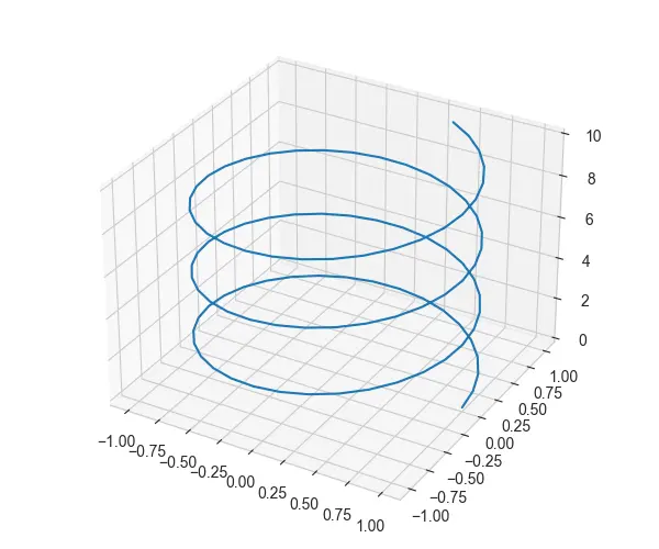
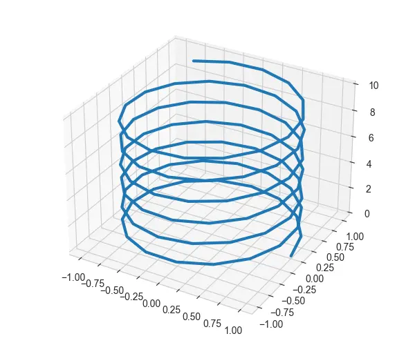
Matplotlib provides an option to create a line plot, and we will create some new data to show off. We will need to create z, a linear space from 0 to 10, and then create x and y based on the cosine and sine of the z-axis.
In the same way as scatter3D() we call plot3D(), this will give us a line plot.
import seaborn as sb
import matplotlib.pyplot as plot
import numpy as np

sb.set_style("whitegrid")

OMEGA = 2

Z1 = np.linspace(0, 10, 100)
X1 = np.cos(OMEGA * Z1)
Y1 = np.sin(OMEGA * Z1)

plot.figure(figsize=(6, 5))
axes = plot.axes(projection="3d")
axes.plot3D(X1, Y1, Z1)
# keeps padding between figure elements
plot.tight_layout()
plot.show()
Now we have a nice spiral forming plot represented in three-dimensional space.
We can style this line using the same keywords for a 2-dimensional plot. Suppose we can change our line width and make this spiral a bit darker.
The argument called OMEGA basically controls how many spirals we want to see in our plot.
import seaborn as sb
import matplotlib.pyplot as plot
import numpy as np

sb.set_style("whitegrid")

OMEGA = 4

Z1 = np.linspace(0, 10, 100)
X1 = np.cos(OMEGA * Z1)
Y1 = np.sin(OMEGA * Z1)

plot.figure(figsize=(6, 5))
axes = plot.axes(projection="3d")
axes.plot3D(X1, Y1, Z1, lw=3)
# keeps padding between figure elements
plot.tight_layout()
plot.show()
Now we can see more thick spirals in our figure.
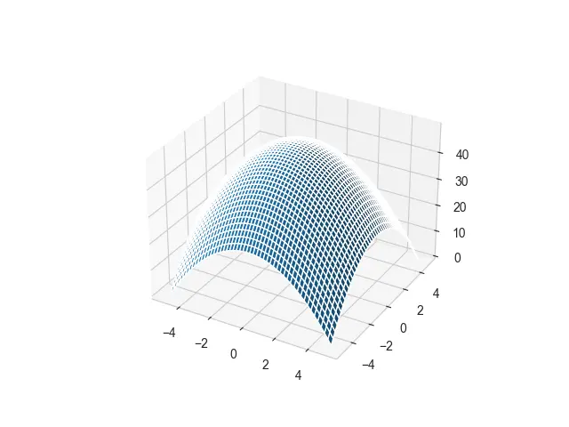
We can also use Matplotlib to create 3-dimensional surfaces and wireframes.
Let’s create a FUNC_Z() function. It will take the x and y values and return the function that we will plot to the surface.
def FUNC_Z(x, y):
    return 50 - (x ** 2 + y ** 2)
We use linspace to create 50 intervals between -5 and 5 for x and y. We need to create a grid instead of having just x and y values.
We can create it using the meshgrid() function. We need to pass it x and y values so that it will repeat them.
X1, Y1 = np.meshgrid(X_VAL, Y_VAL)
Complete code:
import seaborn as sb
import matplotlib.pyplot as plot
import numpy as np


def FUNC_Z(x, y):
    return 50 - (x ** 2 + y ** 2)


sb.set_style("whitegrid")
N = 50

X_VAL = np.linspace(-5, 5, N)
Y_VAL = np.linspace(-5, 5, N)

X1, Y1 = np.meshgrid(X_VAL, Y_VAL)

Z1 = FUNC_Z(X1, Y1)

axes = plot.axes(projection="3d")
axes.plot_surface(X1, Y1, Z1)
plot.show()
Output:
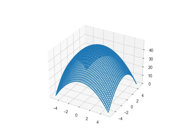
Let’s create a wireframe plot using the plot_wireframe() function. This code is going to look very similar to the surface.
import seaborn as sb
import matplotlib.pyplot as plot
import numpy as np


def FUNC_Z(x, y):
    return 50 - (x ** 2 + y ** 2)


sb.set_style("whitegrid")
N = 50

X_VAL = np.linspace(-5, 5, N)
Y_VAL = np.linspace(-5, 5, N)

X1, Y1 = np.meshgrid(X_VAL, Y_VAL)

Z1 = FUNC_Z(X1, Y1)

axes = plot.axes(projection="3d")
axes.plot_wireframe(X1, Y1, Z1)
plot.show()
Now we have a wireframe rather than a surface, which does not have the middle part filled.
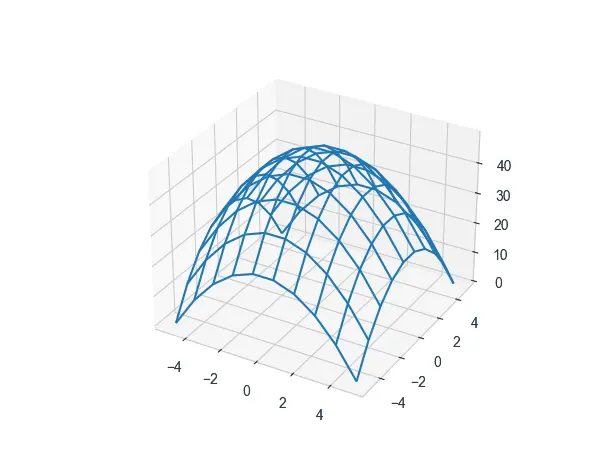
We can change the aesthetics of this wireframe if we change the number of points on our grid.
import seaborn as sb
import matplotlib.pyplot as plot
import numpy as np


def FUNC_Z(x, y):
    return 50 - (x ** 2 + y ** 2)


sb.set_style("whitegrid")
N = 10

X_VAL = np.linspace(-5, 5, N)
Y_VAL = np.linspace(-5, 5, N)

X1, Y1 = np.meshgrid(X_VAL, Y_VAL)

Z1 = FUNC_Z(X1, Y1)

axes = plot.axes(projection="3d")
axes.plot_wireframe(X1, Y1, Z1)
plot.show()
It will create a different aesthetic with a lot more space because we have changed the size of our grid. We also have an option of taking our mouse, clicking on this figure, and dragging it around.

Hello! I am Salman Bin Mehmood(Baum), a software developer and I help organizations, address complex problems. My expertise lies within back-end, data science and machine learning. I am a lifelong learner, currently working on metaverse, and enrolled in a course building an AI application with python. I love solving problems and developing bug-free software for people. I write content related to python and hot Technologies.
LinkedIn