How to Detect Shape in OpenCV

This tutorial shows how to prepare an image, find its external contours, approximate each contour as a polygon, and use the vertex count as a simple shape-classification heuristic with OpenCV.

Prepare a Binary Image for Shape Detection

findContours() works from a binary mask. For the workflow below, foreground shapes are white (255) and the background is black (0). Convert a BGR image to grayscale with cvtColor(), then use threshold() with Otsu’s method to choose a threshold from the image. If the foreground is dark against a light background, invert the resulting mask or use an inverse threshold so the objects are white.

For an input file, load it with cv2.imread("shape-detection.webp") and check that the returned image is not None before processing. Convert the BGR image to grayscale, then make a binary mask with cv2.threshold(gray, 0, 255, cv2.THRESH_BINARY + cv2.THRESH_OTSU). The mask should show foreground objects as white on a black background; use an inverse threshold when the image has the opposite polarity.

Detect and Classify Shapes with findContours() and approxPolyDP()

Call findContours() with RETR_EXTERNAL to retrieve each white object’s outer contour, then use approxPolyDP() and count the resulting vertices. Three vertices suggest a triangle, four suggest a quadrilateral, and five suggest a pentagon. These are heuristics: four vertices do not establish that a shape is a square. More than 12 vertices can label a contour as circle-like; that cutoff depends on approximation tolerance, image resolution, and contour quality.

The short example makes the vertex-count labels clear with representative counts. The complete example that follows loads shape-detection.webp from the same directory as the script, even when launched from another working directory. It prints one heuristic label per contour and, when drawing is enabled, saves an annotated PNG in the current working directory. Install OpenCV with python -m pip install opencv-python before running the image example. The supplied runtime evidence covers only the short label example, not the OpenCV image-processing workflow.

def label_for_vertex_count(count):
    if count == 3:
        return "triangle"
    if count == 4:
        return "quadrilateral"
    if count == 5:
        return "pentagon"
    if count > 12:
        return "circle-like"
    return "polygon"


approximated_vertex_counts = [3, 4, 5, 16]
for count in approximated_vertex_counts:
    print(f"{label_for_vertex_count(count)}: {count} vertices")

triangle: 3 vertices
quadrilateral: 4 vertices
pentagon: 5 vertices
circle-like: 16 vertices

The short snippet isolates the classification rule. This complete script applies the same rule to the supplied image, checks image loading, converts the BGR pixels to grayscale, and builds an Otsu binary mask. The mask assumes bright foreground objects on a darker background; use cv2.THRESH_BINARY_INV when the foreground is dark against a light background. The supplied image contains several panels, so external contours can include panel boundaries as well as the shapes. Labels remain heuristics: four vertices indicate a quadrilateral, not necessarily a square, and contour order and vertex counts depend on image quality and approximation tolerance.

from pathlib import Path


def label_for_vertex_count(count):
    if count == 3:
        return "triangle"
    if count == 4:
        return "quadrilateral"
    if count == 5:
        return "pentagon"
    if count > 12:
        return "circle-like"
    return "polygon"


def main():
    try:
        import cv2
    except ImportError:
        print("OpenCV is required; install it with python -m pip install opencv-python.")
        raise SystemExit(1)

    image_path = Path(__file__).resolve().with_name("shape-detection.webp")
    image = cv2.imread(str(image_path))
    if image is None:
        print(f"Could not load image: {image_path}")
        raise SystemExit(1)

    gray = cv2.cvtColor(image, cv2.COLOR_BGR2GRAY)
    _, mask = cv2.threshold(
        gray, 0, 255, cv2.THRESH_BINARY + cv2.THRESH_OTSU
    )
    result = cv2.findContours(
        mask, cv2.RETR_EXTERNAL, cv2.CHAIN_APPROX_SIMPLE
    )
    contours = result[0] if len(result) == 2 else result[1]

    draw = True
    annotated = image.copy()
    for contour in contours:
        perimeter = cv2.arcLength(contour, True)
        approximation = cv2.approxPolyDP(
            contour, 0.01 * perimeter, True
        )
        label = label_for_vertex_count(len(approximation))
        print(f"{label}: {len(approximation)} vertices")

        if draw:
            cv2.drawContours(
                annotated, [approximation], -1, (0, 0, 255), 2
            )

    if draw:
        output_path = Path.cwd() / "shape-detection-annotated.png"
        if cv2.imwrite(str(output_path), annotated):
            print(f"Saved annotated image: {output_path}")
        else:
            print(f"Could not save annotated image: {output_path}")
            raise SystemExit(1)


if __name__ == "__main__":
    main()

OpenCV color tuples use BGR order, so (0, 0, 255) draws red. A thickness of 2 draws an outline; a negative thickness fills a contour.

Draw Detected Shapes with drawContours()

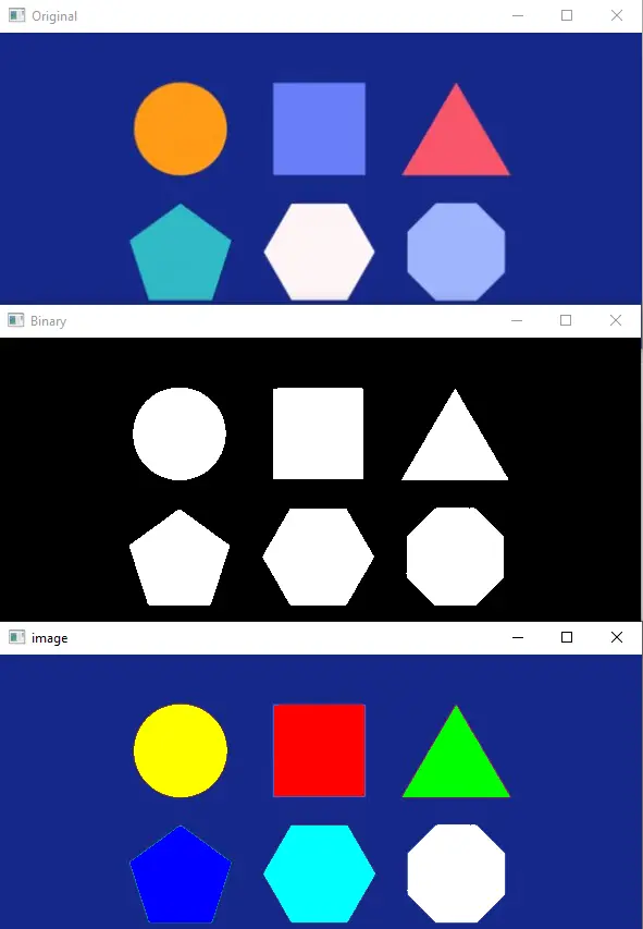
In the complete script, draw = True draws each approximated contour in red and saves shape-detection-annotated.png in the current working directory; cv2.imwrite() reports whether the save succeeded. Set draw = False to skip both drawing and saving. The script does not open a GUI, so it can run in a headless environment. The illustration below remains a visual reference.

Understand the OpenCV Contour Function Arguments

findContours(mask, cv2.RETR_EXTERNAL, cv2.CHAIN_APPROX_SIMPLE) takes the binary mask, a retrieval mode, and a contour-approximation method. RETR_EXTERNAL returns only outer boundaries, which is useful when internal holes are not part of the task. CHAIN_APPROX_SIMPLE compresses straight runs of contour points while preserving the boundary shape. OpenCV versions differ in how many values findContours() returns, so code that supports both forms can select the contours with result[0] if len(result) == 2 else result[1].

approxPolyDP(contour, epsilon, closed) takes a contour, a maximum approximation distance, and a boolean indicating whether the curve is closed. A common choice is 0.01 * cv2.arcLength(contour, True) for epsilon; increasing that proportion generally produces fewer vertices, while decreasing it follows the contour more closely. The function uses the Douglas–Peucker algorithm, so vertex counts depend on both this tolerance and the image.

For drawContours(image, contours, contour_index, color, thickness), the image is modified in place, contours supplies the boundaries, contour_index selects one contour (or -1 for all), and color is a BGR tuple. A negative thickness fills the selected contour.