How to Detect Edge in Python OpenCV

Edge detection is widely used in image processing for background removal, shape detection, and image structure analysis. In an image, an edge is a sudden change in pixel intensity level.

For example, if there is a picture of a cat with a black background, there will be a sudden change in pixel value, from black to white, at the outline of the cat.

OpenCV offers two methods to detect the edges present in an image: a Canny edge detector, which runs a complete multistage pipeline and returns a thin binary edge map, and a Sobel edge detector, which computes the image derivative in a chosen direction and leaves the filtering to you. This tutorial will discuss detecting edges in an image using the Canny or Sobel edge detector in OpenCV.

Both detectors look for the same thing: a derivative of the pixel values that is large where the intensity jumps. You can see the idea with a single row of grayscale values in plain Python, no OpenCV needed.

Run this example:

pixels = [20, 20, 20, 20, 200, 200, 200, 200]
response = [pixels[i + 1] - pixels[i - 1] for i in range(1, len(pixels) - 1)]
print("response:", response)
print("peak:", max(response))

response: [0, 0, 180, 180, 0, 0]
peak: 180

The two non-zero values mark the position of the intensity step. Edge detectors compute a similar response across the whole image, in both directions, and then decide which responses count as real edges.

OpenCV Canny Edge Detection

We can use the Canny() function of OpenCV for Canny edge detection. The function expects a grayscale image, and smoothing it first with the GaussianBlur() function gives a better result. Sudden changes in pixel intensity caused by noise can be detected as extra edges that are not part of the real structures we want to detect, so removing the noise present in the image matters.

The example below builds a small grayscale test image so it runs on its own once OpenCV is installed (pip install opencv-python). It is shown as source rather than executed output; for a real photo, load it with cv2.imread("cat.jpg") and convert it with cv2.cvtColor(img, cv2.COLOR_BGR2GRAY) before smoothing. The result is saved with cv2.imwrite(); on a desktop machine you can display it in a window with cv2.imshow() and cv2.waitKey(0) instead.

import os
import tempfile

try:
    import cv2
    import numpy as np
except ModuleNotFoundError:
    print("this example needs the opencv-python package")
    raise SystemExit(0)

img_src = np.zeros((240, 320), dtype=np.uint8)
cv2.rectangle(img_src, (40, 40), (200, 200), 120, -1)
cv2.circle(img_src, (240, 120), 50, 220, -1)

blur_img = cv2.GaussianBlur(img_src, (3, 3), 0)
img_edges = cv2.Canny(image=blur_img, threshold1=50, threshold2=155)

out_path = os.path.join(tempfile.gettempdir(), "canny-edges.png")
cv2.imwrite(out_path, img_edges)
print("edge map:", img_edges.shape, img_edges.dtype)

On a machine with OpenCV installed, the script writes canny-edges.png to the temp directory and prints edge map: (240, 320) uint8. The output of Canny() is a single-channel 8-bit image in which edge pixels are 255 and everything else is 0. Applied to a photograph, the result looks like this:

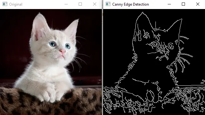
The original photo and the thin white edge map returned by Canny().

The Canny edge detector is multistage and goes through several steps to find the edges present in an image. In the first step, the algorithm reduces the noise present in the given image with a Gaussian filter.

In the second step, the algorithm finds the first derivative of the image in the x and y directions, and from this derivative it computes the magnitude and direction of the edge gradient at each pixel.

In the third step, the algorithm applies non-maximum suppression: it keeps only the pixels that are local maxima along the gradient direction, which thins the detected edges down to single-pixel lines.

In the fourth step, the algorithm filters the edges using the two intensity levels defined by the user, a step called hysteresis thresholding. Pixels with a gradient above the upper level are kept as strong edges, pixels below the lower level are discarded, and pixels between the two levels survive only when they are connected to a strong edge.

In the above code, the first argument image of the Canny() function is the given image, which should be 8-bit. The second argument threshold1 and the third argument threshold2 set the lower and upper levels of that hysteresis range.

The Canny() function also has two optional arguments. The first optional argument, apertureSize, sets the aperture size for the internal Sobel operator used to compute the gradient, and by default its value is 3.

The second optional argument, L2gradient, sets how the gradient magnitude is computed. By default it is False and the faster L1 norm is used; setting it to True selects the more accurate L2 norm.

Changing the threshold range changes the output because the range filters the edges. Raising both thresholds returns fewer, more confident edges, while lowering them returns more edges, including faint or noisy ones.

OpenCV Sobel Edge Detection

The Canny edge detector is multistage, as discussed above: it removes the noise, finds the edges, and filters them using the threshold range. If we want the raw derivatives instead, for example to build custom filtering on top, we can use the Sobel() function of OpenCV. The Sobel() function finds the derivative of an image in the x direction, the y direction, or both, by convolving the image with a derivative kernel, and it does not denoise or threshold the result for us.

The Sobel() function also finds the edges using the sudden change in pixel intensity. The example below computes the x and y derivatives separately so each variable name matches what it holds; like the Canny listing, it needs opencv-python installed and is shown as source rather than executed output. Because ddepth is cv2.CV_64F, the results are signed: a light-to-dark transition produces a value with the opposite sign to a dark-to-light one. cv2.convertScaleAbs() takes the absolute value and converts the result back to 8-bit so the derivative images can be saved or displayed, and cv2.addWeighted() merges both directions into one combined edge response.

import os
import tempfile

try:
    import cv2
    import numpy as np
except ModuleNotFoundError:
    print("this example needs the opencv-python package")
    raise SystemExit(0)

img_src = np.zeros((240, 320), dtype=np.uint8)
cv2.rectangle(img_src, (40, 40), (200, 200), 120, -1)
cv2.circle(img_src, (240, 120), 50, 220, -1)

blur_img = cv2.GaussianBlur(img_src, (3, 3), 0)
sobel_x = cv2.Sobel(src=blur_img, ddepth=cv2.CV_64F, dx=1, dy=0, ksize=3)
sobel_y = cv2.Sobel(src=blur_img, ddepth=cv2.CV_64F, dx=0, dy=1, ksize=3)
sobel_xy = cv2.addWeighted(cv2.convertScaleAbs(sobel_x), 0.5,
                          cv2.convertScaleAbs(sobel_y), 0.5, 0)

out_path = os.path.join(tempfile.gettempdir(), "sobel-edges.png")
cv2.imwrite(out_path, sobel_xy)
print("derivative:", sobel_x.dtype, sobel_x.shape)
print("combined:", sobel_xy.dtype, sobel_xy.shape)

A normal desktop run prints derivative: float64 (240, 320) and combined: uint8 (240, 320), and writes sobel-edges.png to the temp directory. Here sobel_x measures the intensity change along the x (horizontal) direction, so it highlights vertical edges, while sobel_y measures the change along the y direction and highlights horizontal edges; sobel_xy combines both directions. If we display or save the raw CV_64F derivative directly, the signed values saturate and the window fills with dense, noisy speckles rather than clean lines:

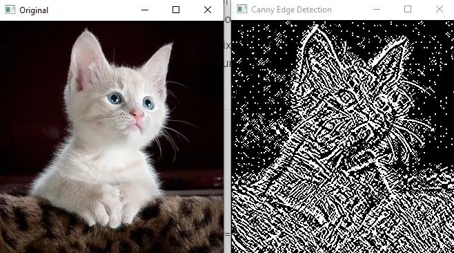
A raw signed Sobel result saturates when displayed, which is why it looks so much busier than the Canny edge map.

The first argument src of the Sobel() function is the source image. The second argument, ddepth, sets the depth of the output image; use cv2.CV_64F or cv2.CV_16S so that signed derivatives are preserved instead of being truncated to 0.

The third argument, dx, sets the order of the x derivative, and the fourth argument, dy, sets the order of the y derivative: dx=1, dy=0 takes the horizontal derivative, highlighting vertical edges; dx=0, dy=1 takes the vertical derivative, highlighting horizontal edges; and dx=1, dy=1 responds to diagonal changes.

The fifth argument, ksize, sets the kernel size, and its value should be 1, 3, 5, or 7 (-1 selects the Scharr operator). The sixth argument, scale, is an optional scale factor for the derivative values, and by default no scale is used.

The seventh argument, delta, is also optional and sets a constant value added to the output. The eighth argument, borderType, is also optional and sets the method for pixel extrapolation, and by default the border type is set to BORDER_DEFAULT.

Check this link for more details about the border types.

Choose Sobel() when you need directional gradient data or want to run your own post-processing; choose Canny() when you want a clean binary edge map with noise suppression and threshold filtering already handled.