HOWTO · SciPy
How to Calculate the Confidence Interval Using SciPy
Learn how to calculate confidence intervals in Python using SciPy, with worked t-distribution and normal-distribution examples whose data and outputs are fully reproducible.
On this page
This article aims to help you calculate the confidence intervals in Python using SciPy. Before we dive into the calculation part, some basic information about the confidence interval needs to be understood.
Calculate the Confidence Interval Using SciPy
When we measure something, we must always calculate the degree of uncertainty in the outcome. A confidence interval is a range of values, calculated from sample data, that is built to contain the true value of the quantity being estimated — for example, a population mean.
Assume you inquire about one’s height. One could tell you that he’s 1.55 meters tall, but that doesn’t tell you anything about the uncertainty of this measurement.
Scientists often want a 95% confidence interval, but 90% or even 99% is also frequent. So, if you ask for the height, one should give you an estimate or a confidence interval, such as: with 95% confidence, the mean height lies between 1.50 meters and 1.60 meters.
The confidence level describes the procedure, not any single result. The true population value is fixed; it is the interval that varies from sample to sample. A 95% confidence level means that if the same procedure were repeated on many samples, about 95% of the intervals produced would contain the true value. A single calculated interval either contains the true value or it does not — the level is a statement about the long-run coverage of the method, not a probability for that one interval.
To calculate the confidence interval, we have to use the following formula:
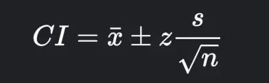
Where:
- The
x_baris the sample mean. - The
zis the confidence level value (the critical value for the chosen level). - The
nis the sample size. - The
sis the sample standard deviation.
Which distribution supplies the critical value depends on what is known about the population standard deviation, not on a fixed sample-size cutoff. When the standard deviation is estimated from the sample itself, the t-distribution accounts for that extra uncertainty through its degrees of freedom, and SciPy’s t.interval() builds the interval from the sample mean and the standard error of the mean. When the interval is built directly from a normal distribution with a given mean and scale, norm.interval() is the corresponding call. The two examples below use one each; both are computed with SciPy 1.18, and every reported value below is the output of the code shown.
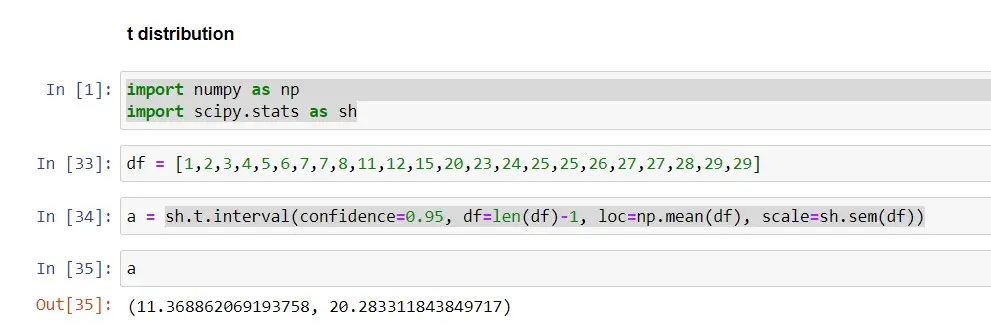
The t-distribution example (n=23). Suppose we have data collected from different villages, a sample of 23 values. We calculate its 95% confidence interval using the t.interval() method, with the confidence parameter set to 0.95, df set to the degrees of freedom (n − 1), loc set to the sample mean, and scale set to the standard error of the mean:
import numpy as np
import scipy.stats as stats

data = [1, 2, 3, 4, 5, 6, 7, 7, 8, 11, 12, 15, 20, 23, 24, 25, 25, 26, 27, 27, 28, 29, 29]

ci_95 = stats.t.interval(confidence=0.95, df=len(data) - 1, loc=np.mean(data), scale=stats.sem(data))
print(tuple(float(v) for v in ci_95))
Output:
(11.368862069193735, 20.28331184384974)
Let’s see the difference in confidence level when we use 99%:
ci_99 = stats.t.interval(confidence=0.99, df=len(data) - 1, loc=np.mean(data), scale=stats.sem(data))
print(tuple(float(v) for v in ci_99))
Output:
(9.767939107911449, 21.884234805132028)

With a 95% confidence interval, the interval is (11.37, 20.28), whereas with a 99% confidence interval, the interval is (9.77, 21.88). Comparing both intervals, we can see that the interval is wider when we use a CI of 99%: demanding that the procedure capture the true value more often requires a wider range. It does not mean there is a 99% probability that this particular interval contains the true value; it means the method that produced it succeeds 99 times out of 100 in the long run.
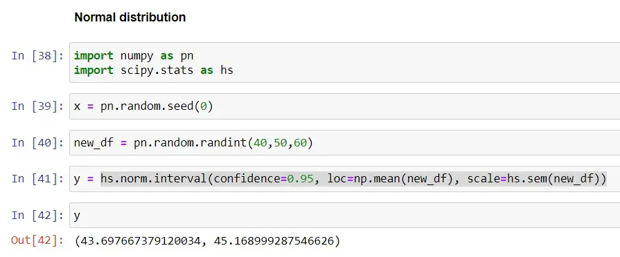
The normal-distribution example (n=60). For a larger dataset, we use the norm.interval() method with the sample mean as loc and the standard error as scale. The data is generated with a fixed seed, so the example is fully reproducible:
np.random.seed(0)
data = np.random.randint(40, 50, 60)

ci_95 = stats.norm.interval(confidence=0.95, loc=np.mean(data), scale=stats.sem(data))
print(tuple(float(v) for v in ci_95))
Output:
(43.697667379120034, 45.168999287546626)
Let’s see the difference in confidence level when we use 99%:
ci_99 = stats.norm.interval(confidence=0.99, loc=np.mean(data), scale=stats.sem(data))
print(tuple(float(v) for v in ci_99))
Output:
(43.46650438268271, 45.40016228398395)

With a 95% confidence interval, the interval is (43.70, 45.17); with a 99% confidence interval, the interval is (43.47, 45.40). As before, the 99% interval is wider, for the same reason: the higher confidence level is a stronger requirement on the procedure, and it is met by widening the range.
Confidence intervals are simple to compute and can provide data analysts and scientists with valuable information. They provide a powerful error estimate and, when applied appropriately and interpreted correctly, can truly help us extract as much information from our data as possible.