TUTORIAL · Algorithm
Counting Sort
This tutorial introduces the counting sort algorithm.
On this page
Counting sort orders integer values by counting how often each value occurs, then using those frequencies to place values in sorted order. It avoids pairwise comparisons, but its time and memory use depend on the width of the value range. That makes it useful when the range is reasonably small; a sparse range can make it impractical. It is also used as a subroutine in radix sort. The central complexity bound is O(n + k), where n is the number of values and k is the range width.
How Counting Sort Works
Let the input contain n integers. Find its minimum min and maximum max, then allocate k = max - min + 1 counters. The offset min lets the algorithm represent negative values with nonnegative counter indexes:
For an input range from the minimum value to the maximum value, map each value x to count index x - min.
For each input value x, increment count[x - min]. These are frequencies: counter index i represents value min + i. Convert frequencies to cumulative positions by adding each counter to the one before it. After this step, each counter gives the number of input values less than or equal to its represented value, which is the final one-based position of the last occurrence of that value.
To build a stable output for records with keys, scan the input from right to left. Place each record at count[key - min] - 1, then decrement that counter. Scanning in reverse preserves the original order of records that share a key:
When sorting records by a key, scan input from right to left during placement so equal-key records keep their original order.
The algorithm needs no counters for an empty input; return an empty result before looking for a minimum or maximum. A basic integer implementation preserves values, while sorting records requires carrying each record into the output array during placement.
Worked Example: Sorting Values with Counting Sort
Consider the input (6, 3, 2, 7, 4, 5, 4, 2). Its minimum is 2, its maximum is 7, and the range width is k = 7 - 2 + 1 = 6. Counter indexes 0 through 5 represent values 2 through 7.
| Value | 2 | 3 | 4 | 5 | 6 | 7 |
|---|---|---|---|---|---|---|
| Frequency | 2 | 1 | 2 | 1 | 1 | 1 |
| Cumulative position | 2 | 3 | 5 | 6 | 7 | 8 |
For example, count[4 - 2] is 2, so the value 4 occurs twice. After accumulation, the counter for 4 is 5: the last 4 belongs at zero-based output index 4. Decrementing its position reserves the preceding slot for the other 4. Repeating this placement for the remaining values produces (2, 2, 3, 4, 4, 5, 6, 7).
The following diagram uses distinct record labels to show how the offset, frequency counts, cumulative positions, and reverse placement fit together. Its example includes a negative key and shows that equal-key records retain their input order.
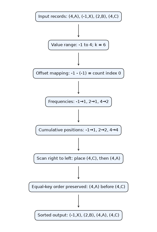
Diagram: the range -1 through 4 maps to six count indexes; frequencies become cumulative positions, and reverse placement keeps (4,A) before (4,C) in the output.
Implement Counting Sort in C++
This complete C++ example returns a new vector, supports signed integers through offset indexing, and handles a vector with no elements before finding its range. It uses standard containers rather than variable-length arrays.
Run this example:
#include <algorithm>
#include <cstddef>
#include <iostream>
#include <vector>

std::vector<int> countingSort(const std::vector<int>& values) {
    if (values.size() == 0) {
        return {};
    }

    const auto bounds = std::minmax_element(values.begin(), values.end());
    const long long minValue = *bounds.first;
    const long long maxValue = *bounds.second;
    const std::size_t range = static_cast<std::size_t>(maxValue - minValue + 1);
    std::vector<std::size_t> count(range, 0);

    for (int value : values) {
        const std::size_t index = static_cast<std::size_t>(value - minValue);
        ++count[index];
    }

    for (std::size_t i = 1; i < count.size(); ++i) {
        count[i] += count[i - 1];
    }

    std::vector<int> output(values.size());
    for (std::size_t i = values.size(); i-- > 0;) {
        const int value = values[i];
        const std::size_t index = static_cast<std::size_t>(value - minValue);
        output[--count[index]] = value;
    }
    return output;
}

int main() {
    const std::vector<int> input{6, 3, 2, 7, 4, 5, 4, 2};
    const std::vector<int> sorted = countingSort(input);

    std::cout << "Input: ";
    for (int value : input) {
        std::cout << value << ' ';
    }
    std::cout << "\nSorted: ";
    for (int value : sorted) {
        std::cout << value << ' ';
    }
    std::cout << '\n';
}
The sample prints the input and the sorted values when compiled and run. This implementation sorts integers; to sort records stably, store the full record in output at the same calculated position rather than storing only its key.
Complexity and When to Use Counting Sort
Finding the range, counting values, accumulating positions, and placing values each take linear time in their respective input or range. The total time is O(n + k). The auxiliary space is also O(n + k) for the counters and output vector. Here k = max - min + 1, so the cost depends on the distance between the minimum and maximum values, not only on how many values appear.
Use counting sort when values are integers and the range is small enough for k counters and an output of n items. For example, a large collection of scores drawn from a compact fixed range can suit it well. A small input spread across a huge range may require too much memory and initialization time, even when most values never occur; a comparison sort or radix sort may then be a better choice. The counter vector must fit available memory, so estimate the range width before allocating it.