TensorFlow Gradient Tape

TensorFlow has played a vital role in being a consistent framework and a compatible work zone for the dynamic machine learning and deep learning field.

One of the most hyped domains is the neural network, and its working principle can be demonstrated easily with the help of the gradient descent algorithm. And TensorFlow assures almost all the libraries required to enhance this experience.

According to the basic concept, the neural network is how the human brain cell operates, decides, recognizes, and functions. Our processing unit can only memorize the information fed at a time.

Rather it follows a learning rate and revises back to back based on dealing with situations. In this process, there is an important term called the cost function or loss function or partial derivative or the basic term gradient.

To visualize the concept, we have tried to demonstrate a common concept, the “Linear Regression” model. If you are not a newbie to machine learning, then we assume you are already familiar with it.

What this model does is extract a relationship between the independent and dependent variables with the help of a regression line.

While establishing the regression line, it is required to know the sum of square errors (SSE), which is the gradient for this particular case. We expect the SSE to be the minimum when we train our model.

The constant process only avails this of training. Here, we calculate the output from our specified equation and reinitialize the driver values with the gradient x learning rate.

The learning rate ensures stability so that our loss function doesn’t show abrupt consequences.

We will update the base values depending on the gradients after initiating a base value. This backward pass is necessary to check if the model was trained properly.

And the gradient tape is just that component that successively stores the cost function along with the updated inputs and outputs. So we get a complete picture of the whole procedure with the detail of the values.

Let’s visualize the method with an example.

Use of Gradient Tape in TensorFlow

In this section, we will not do a theoretical overview. Rather we will follow up on the practical codes and try to demonstrate how we rely on the gradient tape.

So, let’s jump on to the code bases. We are using Google Colab for our instance.

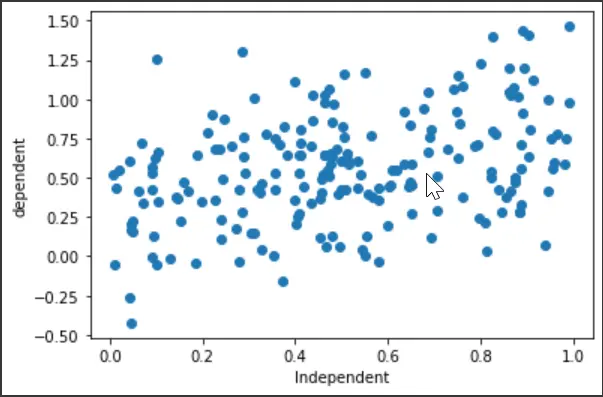
Initially, we will set the library imports and generate a random dataset for the drive. We will also plot a scatter plot to see how the variables behave.

# Necessary Imports
import numpy as np
import tensorflow as tf
import matplotlib.pyplot as plt
import os

# Generating random data
x = np.random.uniform(0.0, 1.0, (200))
y = 0.3 + 0.5 * x + np.random.normal(0.0, 0.3, len(x))
# x
# y

plt.scatter(x, y)
plt.xlabel("Independent")
plt.ylabel("dependent")
plt.show()

Output:

The next code fences will include the regression model and the loss functions declaration. The important part to focus on is that the regression model outputs the predicted value for the dependent variable y, and the equation goes like this:

Here, x is the independent variable, aka the model’s input. Mainly, we will try to see if we have the minimum error between the given y and predicted y^.

The loss function includes the sum of square error (SSE):

# The following equation for the model is ---->  y" = a + b * x
# Linear Regression
class regression:
    def __init__(self):
        self.a = tf.Variable(initial_value=0, dtype=tf.float32)
        self.b = tf.Variable(initial_value=0, dtype=tf.float32)

    def __call__(self, x):
        x = tf.convert_to_tensor(x, dtype=tf.float32)
        y_est = tf.add(self.a, tf.multiply(self.b, x))
        return y_est

model = regression()

# The loss function/ Cost function/ Optimization function (sum of square error)
def loss_func(y_true, y_pred):
    # both y_true and y_pred are tensors
    sse = tf.reduce_sum(tf.square(tf.subtract(y_true, y_pred)))
    return sse

Next, we will define the training section, including the gradient tape. The equation to update the variables a and b are:

# Gradient Descent ----> a = ai - sse * lr (learning rate)
#                                      b = bi - sse * lr


def train(model, inputs, outputs, lr):
    # convert outputs to tensor
    y_true = tf.convert_to_tensor(outputs, dtype=tf.float32)

    # Gradient Tape
    with tf.GradientTape() as g:
        y_pred = model(inputs)
        current_loss = loss_func(y_true, y_pred)

    # slopes/ partal_differentiation/ gradients
    da, db = g.gradient(current_loss, [model.a, model.b])

    # update values

    model.a.assign_sub(da * lr)
    model.b.assign_sub(db * lr)

The next segment is to set the regression line. We will set some epochs for better learning.

We have examined the saturated point and the necessary epoch value for which the loss function is the minimum. Let’s plot the epoch and cost values to see how the output occurred from the whole training section.

# Fitting
def plotting(x, y):
    plt.scatter(x, y)  # scatter
    plt.plot(x, model(x), "r--")

model = regression()
a_val = []
b_val = []
cost_val = []

# epochs
epochs = 70

# learning rate
lr = 0.001

for e in range(epochs):
    a_val.append(model.a)
    b_val.append(model.b)

    # prediction values and errors
    y_pred = model(x)
    cost_value = loss_func(y, y_pred)
    cost_val.append(cost_value)

    # Train
    train(model, x, y, lr)
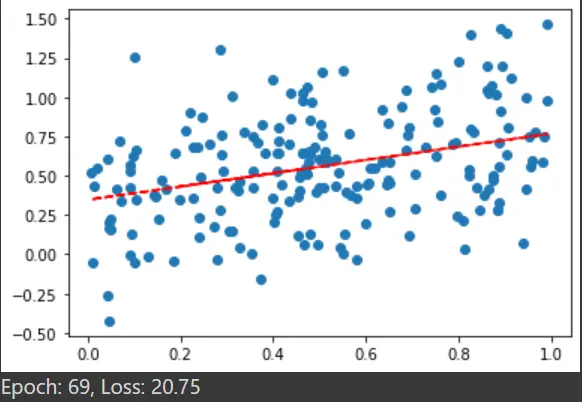
    plotting(x, y)
    plt.show()
    print("Epoch: %d, Loss: %0.2f" % (e, cost_value))

The output scatter-plot from the last epoch:

plt.plot(cost_val)
plt.xlabel("epochs")
plt.ylabel("cost values")

Output:

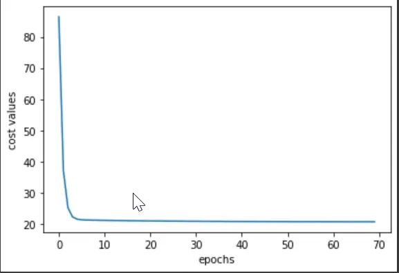
So, it can be said that the cost values reduced drastically in the epoch range of 0-10. And when you run all the epochs, you will notice with the values that the saturated point is near the 64-65 epoch.

Technically, the gradient tape helped collect all the corresponding values, and thus the visualization is more intuitive. You can also preview the whole code in this link.