T Distribution in R

The t-distribution is a probability distribution used to sample a normally distributed population where the sample size is small and the standard deviation is unknown. This tutorial demonstrates how to perform t-distribution in R.

Student’s T Distribution in R

The t-distribution, usually known as the student’s t-distribution, has multiple functions to perform different operations of t-distribution, for example, dt, pt, and qt.

Where dt() is used to find the probability density function of the PDF of the t-distribution with the given random variable, it takes two parameters, one quantile vector and the other is degrees of freedom. The syntax is dt(x, df).

The pt() function gets the cumulative distribution function of the CDF of the t-distribution.

It takes three parameters, the first is the quantile vector, the second is the degrees of freedom, and the third is the lower.trail, which can be true or false. The syntax is pt(q, df, lower.tail = TRUE).

The qt() function gets the inverse cumulative density function of the t-distribution.

It takes three parameters; the first is the vector of probabilities, the second is the degrees of freedom, and the third is the lower.trail. The syntax is qt(p, df, lower.tail = TRUE).

Here is the step-by-step process to perform student t-distribution in R.

Once we know the process now, let’s try to implement the student t-distribution in R. Let’s find the value of t-distribution at x=1 and degrees of freedom 50.

See example:

# value of t-distribution probality density function at x=1 and df = 50
dt(x = 1, df = 50)

The code above will show the value of the t-distribution probability density function at x=1 and df = 50. See output:

[1] 0.2395711

Now let’s find the p-value and confidence interval of t-distribution using the pt() method. See example:

# area to the right of a t-statistic with the value of 3.1 quantile and 30 degrees of freedom
pt(q = 3.1, df = 30, lower.tail = FALSE)

The code above will use the method pt to find the area to the right of a t-statistic with the value of 3.1 quantiles and 30 degrees of freedom. See output:

[1] 0.002092242

We found that the one-sided p-value here is 0.2%. If we want to construct a two-sided 50% confidence interval, we can use the qt() function to find the t-score and t-value for 50% confidence.

# value in each tail is 0.2% and confidence is 50%, we will find 0.2th percentile of t-distribution with 30 degrees of freedom
qt(p = 0.002, df = 30, lower.tail = TRUE)

The qt will find the t-value, which can be used as a critical value for the confidence interval of 50%. See output:

[1] -3.117682

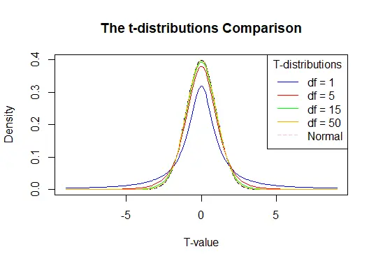
Now let’s compare probability density functions with different degrees of freedom. We do that because it will show the larger the number of degrees of freedom, the closer the plot is to the normal distribution.

See example:

# vector of 200 values between -9 and 9
a <- seq(-9, 9, length = 200)

# Degrees of freedom with maximum 50 degrees
df = c(1,5,15,50)

#plot line colors
colour = c("blue", "red", "green", "orange","pink")

# the normal distribution
plot(a, dnorm(a), type = "l", lty = 2, xlab = "T-value", ylab = "Density",
     main = "The t-distributions Comparison", col = "darkblue")

# Adding t-distributions to the plot
for (i in 1:4){
  lines(a, dt(a, df[i]), col = colour[i])
}

# Adding legend
legend("topright", c("df = 1", "df = 5", "df = 15", "df = 50", "Normal"),
       col = colour, title = "T-distributions", lty = c(1,1,1,1,2))

The code above will show the comparison plot for the t-distributions of different degrees of freedom. See the plot: