How to Perform Time Series Analysis and Forecasts in R

1. Use the ts() Function to Perform Time Series Analysis in R
2. Use the aggregate() Function to Perform Time Series Analysis in R
3. Use the decompose() and stl() Functions to Perform Time Series Analysis in R
4. Other Functions to Perform Time Series Analysis in R
5. Use the predict() Function to Perform Time Series Forecasts in R
6. Conclusion

This article introduces the functions available in base R to analyze a time series and make predictions based on that data.

Use the ts() Function to Perform Time Series Analysis in R

The first step is to create a time series object to conduct time series analysis in R.

Suppose we have the data in a vector, matrix, or data frame. We need to use the ts() function to create a time series object. Only the data is required, not the dates or times associated with it.

Date/time information is usually provided using the start and frequency arguments.

frequency specifies how many observations are there for the unit period. This argument identifies seasonal variations in that period.

Example code:

# CREATE DATA FOR A TIME SERIES.
# A vector of a sequence of integers for the TREND.
set.seed(9797)
s_1 = seq(221:256)

# A cyclic vector for SEASONAL variations.
s_2 = cos(seq(from=1/12*pi, to=6*pi, by=(6*pi/36)))*5

# Random numbers for errors (white noise).
set.seed(65)
s_3 = rnorm(36)

# The data vector.
s = s_1 + s_2 + s_3

# The time series object is created.
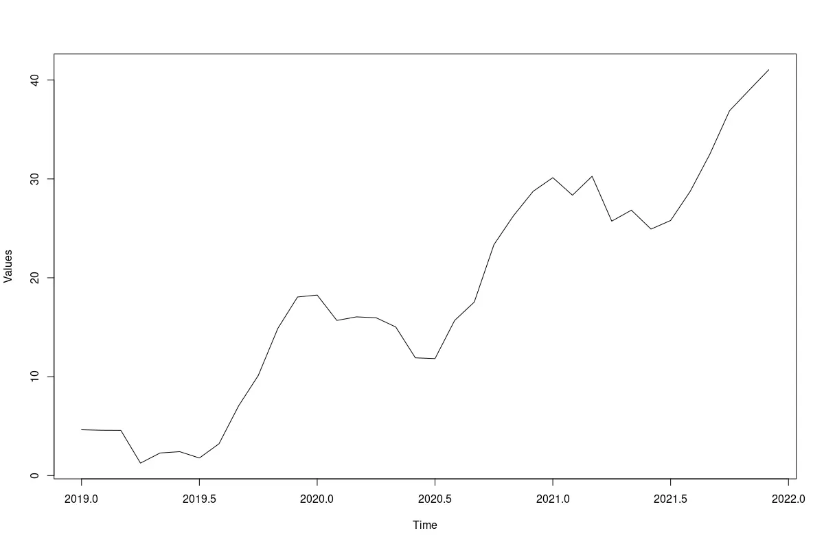
my_t = ts(s, start = c(2019,1), frequency = 12)

# Plot the time series.
plot(my_t, ylab = "Values")

Output:

The plot.ts() function gives more options specific to time series. This is particularly useful for multiple time series.

The time series object created by the ts() function has properties that facilitate further analysis.

Example:

str(my_t)

Output:

Time-Series [1:36] from 2019 to 2022: 4.63 4.58 4.57 1.26 2.29 ...

Use the aggregate() Function to Perform Time Series Analysis in R

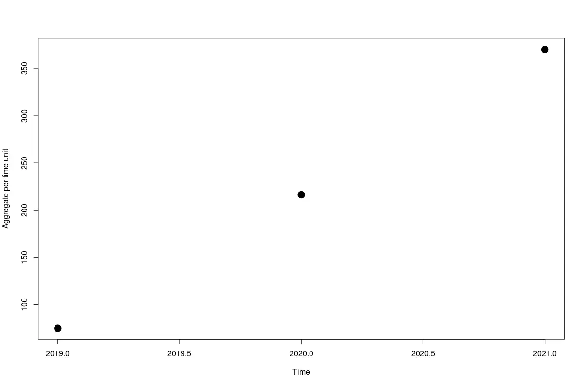
We can aggregate the data per unit to remove the seasonal variations using the aggregate() function if we have data for several time units. We will get one observation for each unit of time.

Example:

plot(aggregate(my_t), type="p", pch=20, cex=3, ylab="Aggregate per time unit")

Output:

To isolate and study the seasonal variations, we can combine corresponding sub-units (such as months) across all units of time (such as years) using the cycle() function. For example, we can differentiate the time series boxplot into its seasonal components.

Use the decompose() and stl() Functions to Perform Time Series Analysis in R

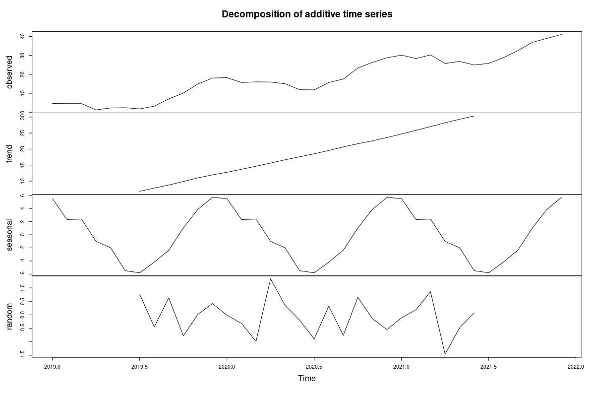
Often, time series have trends, seasonal variations, and random variations. We can statistically break down the data into these three constituent components using the decompose() function.

This function uses moving averages. Depending on the data and our theory, we can specify an additive or multiplicative decomposition.

Example:

plot(decompose(my_t))

Output:

We can use the type="multiplicative" argument in decompose() if we believe the data is multiplicative.

Another function, stl(), uses a different smoothing technique, loess, to isolate the components.

The code plot(stl(ts_object_name, s.window="periodic")) will output a plot produced by such a decomposition.

Other Functions to Perform Time Series Analysis in R

The following are other functions we can use to conduct time series analysis in R.

the acf(), pacf(), and ccf() Functions

We can use the acf() function to estimate the autocorrelation or autocovariance between observations for second-order stationary time series models.

In many cases, this autocorrelation is in the random component of the time series that remains after removing the trend and seasonal components.

We can get the autocorrelation for a particular lag from the vector acf, a list element returned by the function. By default, this function creates a correlogram.

The functions pacf() and ccf() are analogous. They estimate the partial autocorrelations and cross-correlations, respectively.

the nls() Function

The nonlinear least-squares function, nls(), can be used with an appropriate formula to build time series models such as the Bass model for forecasting.

the HoltWinters() Function

The HoltWinters() function computes the Holt-Winters Filtering for the specified ts() object. It estimates the smoothing parameters of the model.

the ar() Function

The ar() function helps us fit an auto-regressive model. It uses the AIC to select the complexity. It supports several optimization methods such as burg, ols, mle, yw.

the arima() Function

The arima() function facilitates modeling both stationary and non-stationary time series data using auto-regressive and moving average methods. It also enables the integration of series created using differencing.

We specify the non-seasonal specifics of the model using a list supplied to the order argument. The seasonal specification is given using the seasonal argument.

Use the predict() Function to Perform Time Series Forecasts in R

Once a model is built, we can employ the predict() function to make forecasts.

Functions specialized for time series forecasts such as predict.Arima(), predict.ar(), and predict.HoltWinters() are also available.

Conclusion

For help with the mentioned functions, access the inbuilt documentation in R. The book Introductory Time Series with R by P.S.P. Cowpertwait and A.V. Metcalfe gives a broad overview of time series modeling with R.