How to Perform K-Means Clustering in Base R

1. About K-Means Clustering in R
2. the kmeans() Function in R
3. K-Means Model in R
4. the Number of Clusters (K)
5. Visualize the Clusters in R
6. Other Practical Considerations
7. References

This article shows how to perform K-means clustering in R. All the steps, including visualization, are demonstrated using base R functions.

About K-Means Clustering in R

K-means clustering is an unsupervised statistical technique that divides the data set into disjoint, homogeneous sub-groups.

We must bear the following points in mind when performing K-means clustering.

1. All variables must be numeric because the method depends on calculating means and distances. Factor data that is coded with numbers is not numeric.
2. There should be no dependent variable in our data set.
3. This method assigns each observation to a cluster. Therefore, it is sensitive to outliers and changes in the data.
4. It works well with disjoint clusters and poorly where the data has overlapping clusters.

the kmeans() Function in R

Base R includes the kmeans() function for K-means clustering.

We will use the following arguments.

1. The first argument is the data.
2. The second argument, centers, is the number of clusters.
3. The third argument, nstart, is the number of times to repeat the clustering with different initial centroids.

The K-means algorithm gives a local optimum for the total within-group sum of squares. This local optimum depends on the randomly chosen initial centroids.

Hence, nstart is used to repeat the clustering. The function returns the clusters with the lowest total.

K-Means Model in R

To create a K-means model, we will create a data frame with two variables and three clusters.

Example Code:

# Vectors for the data frame.
set.seed(4987)
M1 = rnorm(13)
set.seed(9874)
M2 = rnorm(11) + 3
set.seed(8749)
N1 = runif(13)
set.seed(7498)
N2 = runif(11) -2
set.seed(6237)
M3 = rnorm(14) - 6
set.seed(2376)
N3 = runif(14) + 1

# Data frames.
df1 = data.frame(M1, N1)
colnames(df1) = c("M","N")
df2 = data.frame(M2, N2)
colnames(df2) = c("M","N")
df3 = data.frame(M3,N3)
colnames(df3) = c("M","N")

DF = rbind(df1, df2, df3) # Final data frame.

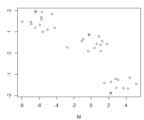
Let us visualize this data.

Example Code:

plot(DF)

The plot of the data frame:

We will now create the K-means model.

Example Code:

# The K-means model.
set.seed(9944)
km_1 = kmeans(DF, centers=3, nstart = 20)

The variable cluster in our model holds the cluster labels the algorithm came up with. The variable tot.withinss holds the total within-group sum of squares.

Let us see the cluster labels that the algorithm assigned. The only thing that matters is that the observations belonging to a cluster should have the same label.

Example Code:

km_1$cluster

Output:

> km_1$cluster
 [1] 1 1 1 1 1 1 1 1 1 1 1 1 1 3 3 3 3 3 3 3 3 3 3 3 2 2 2 2 2 2 2 2 2 2 2 2 2 2

We find that the clusters are identified correctly.

the Number of Clusters (K)

In reality, we may not know the number of clusters our data has. In such a case, we need to try out different values of K and see which value gives a reasonably low total within-group sum of squares.

The problem is, as K increases, we will be creating more centroids close to the data points, and the total within-group sum of squares will drop.

Thus, we need to find a reasonably small K that finds clusters present in the data but does not overfit it.

The usual approach is called the elbow bend method. We create models for different values of K starting from 1 and plot each model’s total within-group sum of squares.

We look for the point in the plot where the slope of the line changes the most. It looks like the elbow joint of an arm. That particular K is chosen for the model.

In the example code, we will use a loop to create models and a vector to store each model’s total within-group sum of squares.

Example Code:

# Create a vector to hold the total within-group sum of squares of each model.
vec_ss = NULL

# Create a loop that creates K-means models with increasing value of K.
# Add the total within group sum of squares of each model to the vector.
for(k in 1:20){
  set.seed(8520)
  vec_ss[k] = kmeans(DF, centers=k, nstart=18)$tot.withinss
}

# View the vector with the total sum of squares of the 20 models.
vec_ss

# Plot the values of the vector.
plot(vec_ss, type="l", xaxp=c(0,20,10), xlab="K", ylab="Total within-group-ss")

Output:

Elbow bend plot to estimate correct K:

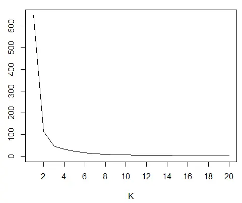
The elbow bend is at K = 3, which is the correct value for our data.

Visualize the Clusters in R

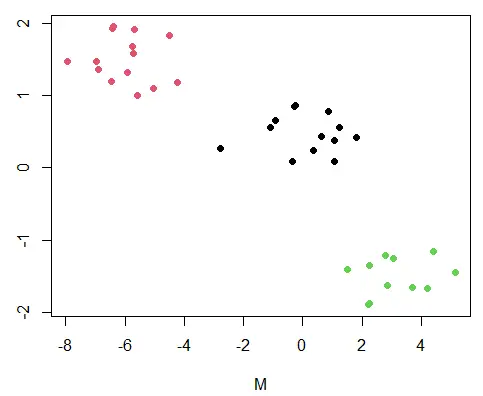
We can visualize the clusters with a scatter plot. The color argument, col, distinguishes the clusters.

The clusters are numbered 1, 2, 3; the col argument picks those colors from the existing palette for the corresponding points.

Example Code:

plot(DF, col=km_1$cluster, pch=19)

Output:

K-means cluster plot.

When there are more than two variables, we can do the following.

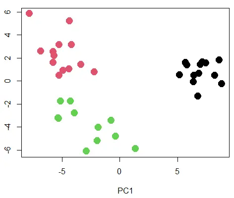
1. Create the K-means model and get the cluster vector.
2. Create a Principal Components model.
3. Plot the first two principal components.

Example Code:

# First, we will add a third variable to our data frame.
O1 = rnorm(13,10,2)
O2 = rnorm(11, 5,3)
O3 = rnorm(14,0,2)
O = as.data.frame(c(O1,O2,O3))
colnames(O) = "O"
DF = cbind(DF, O)

##################################

# The K-means model.
km_2 = kmeans(DF, centers=3, nstart=20)

# The PCA model.
pca_mod = prcomp(DF)

# Visualize the first two principal components with the cluster labels as color.
plot(pca_mod$x[,1:2], col=km_2$cluster, pch=19, cex=2)

Output:

The PCA scatter plot with clusters.

Other Practical Considerations

1. The kmeans() function uses a random number to generate the initial centroids. Using the set.seed() function makes our code reproducible.
2. We must remove observations with missing values to use the kmeans() function. We can use the na.omit() function for this purpose.
3. We may choose to scale each variable to have a mean of 0 and sd of 1 using the scale() function.

References

The book An Introduction to Statistical Learning introduces K-means clustering using R.