How to Test Hypothesis in R

Jesse John Feb 02, 2024

R R Test

t Test in R
Wilcoxon Test in R
Paired t and Wilcoxon Tests in R
Other Tests in the stats Package in R

R provides many functions to perform hypothesis tests.

This article will introduce two functions that will help us perform the t and Wilcoxon tests. We will also see how to discover many other tests built into R.

`t` Test in R

The function t.test() is used for the Student’s t test. The same function can be used for one-sample and two-sample tests and two-tailed and one-tailed tests.

The main arguments are:

x: A vector of numbers.
mu: The unknown value of the mean or the unknown difference of means.
alternative: For one-tailed tests, we should specify either greater or less for the alternate hypothesis.
conf.level: The confidence level of the interval. By default, a level of 0.95 is used.

For two-sample tests, we also use the following:

formula: It is in numeric_vector ~ two-factor_vector form.
data: This data frame should contain the variables mentioned in formula.
var.equal: If TRUE, the variance is computed for the pooled sample. If FALSE(default), the Welch approximation is used.

The output includes the following:

A confidence interval at the given level of confidence around the sample mean.
A p-value stating the probability of the true mean being the specified value mu, given the sample mean.

One-Sample Two-Tailed `t` Test in R

We will now perform one-sample two-tailed t tests on sample data and look at the output.

Example Code:

# Data
# Population Mean = 8; Population SD = 3.
set.seed(3232)
one = rnorm(232,8,3)

# One-sample two-tailed t tests.
# mu is the correct value.
t.test(one, mu = 8)

# mu is some desired value.
# Let us check if mu is 10
t.test(one, mu = 10)

# Change the confidence level.
t.test(one, mu = 10, conf.level = 0.99)

Output:

> # One-sample two-tailed t tests.
> # mu is the correct value.
> t.test(one, mu = 8)

	One Sample t-test
data:  one
t = 0.59131, df = 231, p-value = 0.5549
alternative hypothesis: true mean is not equal to 8
95 percent confidence interval:
 7.741578 8.480045
sample estimates:
mean of x
 8.110811

> # mu is some desired value.
> # Let us check if mu is 10
> t.test(one, mu = 10)

	One Sample t-test
data:  one
t = -10.081, df = 231, p-value < 2.2e-16
alternative hypothesis: true mean is not equal to 10
95 percent confidence interval:
 7.741578 8.480045
sample estimates:
mean of x
 8.110811

When we tested the hypothesis that mu equals 8, we got a very large p-value in the first case. We cannot reject the null hypothesis.

The confidence interval for the sample mean includes the value of mu.

In the second test, the small p-value suggests that the probability of mu being 10 is extremely low. The third case illustrates the syntax for changing the confidence level.

One-Sample One-Tailed `t` Test in R

For a one-tailed test, the argument alternative is used. This is the alternative hypothesis.

Example Code:

# One-sample, one-tailed t test.
t.test(one, mu = 10, alternative = "less", conf.level = 0.99)

# Change mu
t.test(one, mu = 8.3, alternative = "less", conf.level = 0.99)

Output:

> # One-sample, one-tailed t test.
> t.test(one, mu = 10, alternative = "less", conf.level = 0.99)

	One Sample t-test

data:  one
t = -10.081, df = 231, p-value < 2.2e-16
alternative hypothesis: true mean is less than 10
99 percent confidence interval:
     -Inf 8.549816
sample estimates:
mean of x
 8.110811

> # Change mu
> t.test(one, mu = 8.3, alternative = "less", conf.level = 0.99)

	One Sample t-test

data:  one
t = -1.0095, df = 231, p-value = 0.1569
alternative hypothesis: true mean is less than 8.3
99 percent confidence interval:
     -Inf 8.549816
sample estimates:
mean of x
 8.110811

First, we tested the hypothesis that mu is 10 or more and got a low p-value.

We tested the hypothesis that mu is 8.3 or more in the second case. Now the p-value was higher.

Two-Sample `t` Test in R

For the two-sample t test, the data must be in the form of a data frame or a matrix.

It must have both samples in a single numeric vector.
The sample/group must be specified using a two-factor vector.
Therefore, each row of the data frame or matrix contains observation and the group it belongs to.
Depending on which factor is first and second, we need to calculate the difference of the first mean minus the second mean for the argument mu. This is very important.

We will first test the hypothesis that two samples have the same mean. The second test checks whether the means differ by mu.

Example Code:

# Create vectors and data frame.
set.seed(6565)
two_a = rnorm(75, 8, 3.5)
set.seed(9898)
two_b = rnorm(65, 8.5, 3)
two = c(two_a, two_b)
ftr = c(rep("A",75), rep("B",65))
dtf = data.frame(DV = two, FV = ftr)

# Two-sample t test for no difference in means.
t.test(formula=DV~FV, data=dtf)

# Two-sample t test for a difference of mu between the means.
t.test(formula=DV~FV, data=dtf, mu=-1.5)


# Two-sample t test with pooled variance at 90 percent confidence interval.
t.test(formula=DV~FV, data=dtf, var.equal=TRUE, conf.level=0.9)

Output:

> # Two-sample t test for no difference in means.
> t.test(formula=DV~FV, data=dtf)

	Welch Two Sample t-test

data:  DV by FV
t = -2.2723, df = 137.16, p-value = 0.02462
alternative hypothesis: true difference in means between group A and group B is not equal to 0
95 percent confidence interval:
 -2.3975526 -0.1663727
sample estimates:
mean in group A mean in group B
       7.815221        9.097184


> # Two-sample t test for a difference of mu between the means.
> t.test(formula=DV~FV, data=dtf, mu=-1.5)

	Welch Two Sample t-test

data:  DV by FV
t = 0.38648, df = 137.16, p-value = 0.6997
alternative hypothesis: true difference in means between group A and group B is not equal to -1.5
95 percent confidence interval:
 -2.3975526 -0.1663727
sample estimates:
mean in group A mean in group B
       7.815221        9.097184

First, we performed the default two-sample t test, the Welch test, and tested the null hypothesis that the difference of the means is 0. The p-value is about 0.02.

Second, we tested whether the difference in means is -1.5.

The third case illustrates the syntax for the t test, assuming that the two samples have the same variance.

Wilcoxon Test in R

The syntax for the Wilcoxon test is similar.

One-Sample Two-Sided Wilcoxon Test in R

The argument mu is the median as per the null hypothesis we are testing.

Example Code:

# Wilcoxon test.
# One-sample two-tailed test.
wilcox.test(one, mu=8)

# Try a different mu.
wilcox.test(one, mu=9, )

Output:

> wilcox.test(one, mu=8)

	Wilcoxon signed rank test with continuity correction

data:  one
V = 13992, p-value = 0.6408
alternative hypothesis: true location is not equal to 8

> # Try a different mu.
> wilcox.test(one, mu=9, )

	Wilcoxon signed rank test with continuity correction

data:  one
V = 8953, p-value = 8.341e-06
alternative hypothesis: true location is not equal to 9

In the first case, the sample supports the null hypothesis that the median is 8.

In the second case, we get a very small p-value.

Two-Sample Wilcoxon Test in R

This is also called the Mann-Whitney test.

Example Code:

# Test whether two locations differ by mu.
wilcox.test(formula=DV~FV, data=dtf, mu=-1.5)

wilcox.test(formula=DV~FV, data=dtf)

Output:

> # Test whether two two locations differ by mu.
> wilcox.test(formula=DV~FV, data=dtf, mu=-1.5)

	Wilcoxon rank sum test with continuity correction

data:  DV by FV
W = 2530, p-value = 0.7007
alternative hypothesis: true location shift is not equal to -1.5


> wilcox.test(formula=DV~FV, data=dtf)

	Wilcoxon rank sum test with continuity correction

data:  DV by FV
W = 1888, p-value = 0.0218
alternative hypothesis: true location shift is not equal to 0

In the first case, we tested the hypothesis that the location of the two samples differs by -1.5. The large p-value supports the null hypothesis.

We tested the hypothesis that the two samples have the same location in the second case.

Paired `t` and Wilcoxon Tests in R

When data is paired, there are two observations per unit; we should use the paired version of these tests to test the hypothesis that there is no difference, or a specified difference, between the paired observations of the sample.

We will use the argument paired = TRUE for these tests.
The data must be given in two separate numeric vectors of equal length to the arguments x and y.

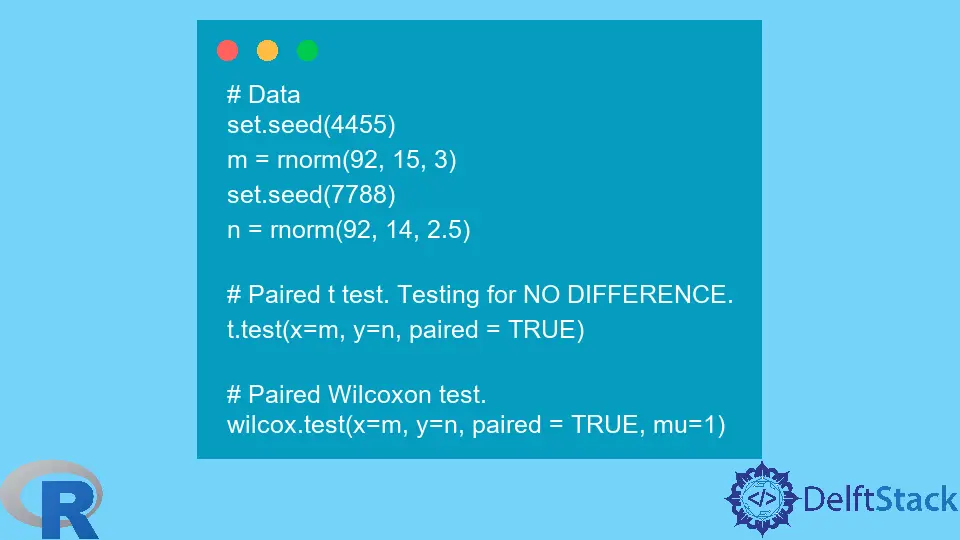
Example Code:

# Data
set.seed(4455)
m = rnorm(92, 15, 3)
set.seed(7788)
n = rnorm(92, 14, 2.5)

# Paired t test. Testing for NO DIFFERENCE.
t.test(x=m, y=n, paired = TRUE)

# Paired Wilcoxon test.
wilcox.test(x=m, y=n, paired = TRUE, mu=1)

Output:

> # Paired t test. Testing for NO DIFFERENCE.
> t.test(x=m, y=n, paired = TRUE)

	Paired t-test

data:  m and n
t = 2.5187, df = 91, p-value = 0.01353
alternative hypothesis: true difference in means is not equal to 0
95 percent confidence interval:
 0.1962145 1.6605854
sample estimates:
mean of the differences
              0.9283999

> # Paired Wilcoxon test.
> wilcox.test(x=m, y=n, paired = TRUE, mu=1)

	Wilcoxon signed rank test with continuity correction

data:  m and n
V = 1930, p-value = 0.4169
alternative hypothesis: true location shift is not equal to 1

In the example of the paired t test, the null hypothesis that the difference is 0 cannot be supported by this sample.

In the paired Wilcoxon test, we tested the hypothesis that the difference is 1. We find the p-value high.

Other Tests in the `stats` Package in R

The default installation of R includes the stats package. This package provides many other functions to test hypotheses about sample statistics.

Run the code below to get a list of all the functions in the package.

Example Code:

library(help = "stats")

R provides documentation and examples for each test function that can be accessed via the inbuilt help.

Author: Jesse John

Jesse is passionate about data analysis and visualization. He uses the R statistical programming language for all aspects of his work.

t Test in R

One-Sample Two-Tailed t Test in R

One-Sample One-Tailed t Test in R

Two-Sample t Test in R

Wilcoxon Test in R

One-Sample Two-Sided Wilcoxon Test in R

Two-Sample Wilcoxon Test in R

Paired t and Wilcoxon Tests in R

Other Tests in the stats Package in R

Related Article - R Test

`t` Test in R

One-Sample Two-Tailed `t` Test in R

One-Sample One-Tailed `t` Test in R

Two-Sample `t` Test in R

Paired `t` and Wilcoxon Tests in R

Other Tests in the `stats` Package in R