How to Imitate Ode45() Function in Python

1. Use SciPy’s solve_ivp() Method to Imitate the ode45() Function of MATLAB in Python
2. Use Custom Integration Scheme to Imitate the ode45() Function of MATLAB in Python
3. Use Scikit-Learn’s Regressor With Interpolation to Imitate the ode45() Function of MATLAB in Python
4. Conclusion

The ode45() function in MATLAB is a versatile ordinary differential equation (ODE) solver that adapts its time step to the behavior of the solution during integration. In Python, there isn’t an exact equivalent, but several libraries and methods can mimic its functionality.

Ordinary differential equations are used in MATLAB to solve many scientific problems. The ode45() is used in MATLAB to solve differential equations.

This article will show how we can imitate the ode45() function. Let’s explore various approaches to emulate the ode45() functionality in Python.

Use SciPy’s solve_ivp() Method to Imitate the ode45() Function of MATLAB in Python

To imitate the ode45() function of MATLAB in Python, we can use the solve_ivp() method defined in the scipy module. The solve_ivp() method integrates a system of ordinary differential equations (ODEs).

The solve_ivp() function from SciPy is a powerful method used for solving initial value problems (IVPs) for ordinary differential equations (ODEs). Its syntax involves several parameters that allow for control over the integration process.

Syntax:

solve_ivp(fun, t_span, y0, method="RK45", t_eval=None, args=None, ...)

The solve_ivp() method takes a function as its first input argument. The function given in the input argument must return an array containing the coefficients of the differential equation.

In the second input argument, the solve_ivp() method takes a tuple or list containing two numerical values. The values represent the interval of integration, where the first value in the tuple represents the start of the interval, and the second value of the tuple represents the highest value in the interval.

In the third input argument, the solve_ivp() method takes an array representing the initial values.

Parameters:

• fun: A callable function. The differential equation function, fun(t, y), where t is the independent variable (time) and y is the dependent variable (state vector).
• t_span: A tuple (t_start, t_end) specifying the initial and final time points for integration.
• y0: The initial state of the system at t_start.
• method='RK45' (optional): The integration method to be used. The default is 'RK45' (explicit Runge-Kutta method of order 5(4)).
• t_eval=None (optional): Time points where the solution should be reported. If specified, the solver will only return the solution at these time points.
• args=None (optional): Additional arguments to be passed to the fun function (fun(t, y, *args)).
• ...: Other parameters. The solve_ivp() function supports other parameters based on the chosen integration method, such as rtol (relative tolerance), atol (absolute tolerance), max_step (maximum step size), etc.

Return Value:

A scipy.integrate.OdeResult object containing the solution to the ODE. It includes attributes such as t (time points), y (solution at corresponding time points), success (Boolean indicating if the integration was successful), and more.

After execution, the solve_ivp() method returns objects with various attributes:

1. The t attribute contains a numpy array containing time points.

2. The y attribute contains a numpy array with values and time points in t.

3. The sol attribute contains an Odesolution object containing the solution of the differential equation. If the dense_output argument is set to false in the solve_ivp() method, the sol attribute contains None.

To understand this better, see the following example:

from scipy.integrate import solve_ivp


def function(t, y):
    return 2 * y


interval = [0, 10]
initial_values = [10, 15, 25]
solution = solve_ivp(function, interval, initial_values)
print("Time:", solution.t)
print("Y:", solution.y)

Output:

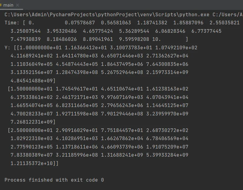
In the above example, we first defined a function named function that takes t and y as its input argument and returns a value based on y.

Then, we have defined an interval and initial values for the ODE using the variables interval and initial_values, respectively. We pass function, interval, and initial_values as input arguments to the solve_ivp() function, and lastly, we get the output in the variable solution.

In the output, you can observe that the time values are spread throughout the interval 0 to 10. Similarly, the output contains a y value corresponding to each time value.

We can also explicitly specify the time points in the attribute t of the solution. For this, we need to pass an array containing the desired time values for which we need the y values to the t_eval argument of the solve_ivp() method, as shown below.

from scipy.integrate import solve_ivp


def function(t, y):
    return 2 * y


interval = [0, 10]
initial_values = [10, 15, 25]
time_values = [1, 2, 3, 6, 7, 8]
solution = solve_ivp(function, interval, initial_values, t_eval=time_values)
print("Time:", solution.t)
print("Y:", solution.y)

Output:

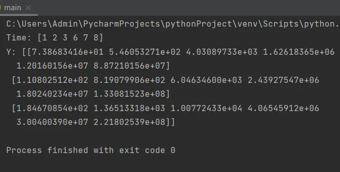
You can see that the time values only contain those values that are passed as input arguments to the t_eval parameter. Similarly, the attribute y contains values for only the specified t values.

This approach can help you obtain values for certain points in the interval.

Use Custom Integration Scheme to Imitate the ode45() Function of MATLAB in Python

Implementing a custom numerical integration method (e.g., Runge-Kutta methods) allows better control over the integration process, similar to ode45().

The Runge-Kutta method is a numerical technique used to solve differential equations. The classic Runge-Kutta method of order 4 (RK4) involves calculating four slopes to estimate the next value.

Example Code:

This code demonstrates an implementation of the fourth-order Runge-Kutta (RK4) method to solve an ordinary differential equation (ODE).

The rk4 function is a numerical solver that uses the RK4 method to approximate the solution to a given ODE.

• func: Represents the function describing the ODE (dy/dt = func(t, y)).
• t_span: A tuple (t_start, t_end) specifying the initial and final time points for integration.
• y0: The initial value of the dependent variable at t_start.
• h: The step size or time increment used for integration.

import numpy as np


def rk4(func, t_span, y0, h):
    t_values = np.arange(t_span[0], t_span[1] + h, h)
    y_values = [y0]
    t = t_span[0]
    y = y0

    for t_next in t_values[1:]:
        k1 = func(t, y)
        k2 = func(t + 0.5 * h, y + 0.5 * h * k1)
        k3 = func(t + 0.5 * h, y + 0.5 * h * k2)
        k4 = func(t + h, y + h * k3)
        y = y + h * (k1 + 2 * k2 + 2 * k3 + k4) / 6
        t = t_next
        y_values.append(y)

    return t_values, np.array(y_values)


def ode_func(t, y):
    return y - t**2 + 1  # Example ODE dy/dt = y - t^2 + 1


t_span = (0, 10)  # Time span
h = 0.1  # Time step
y0 = 0.5  # Initial condition

t_values, y_values = rk4(ode_func, t_span, y0, h)

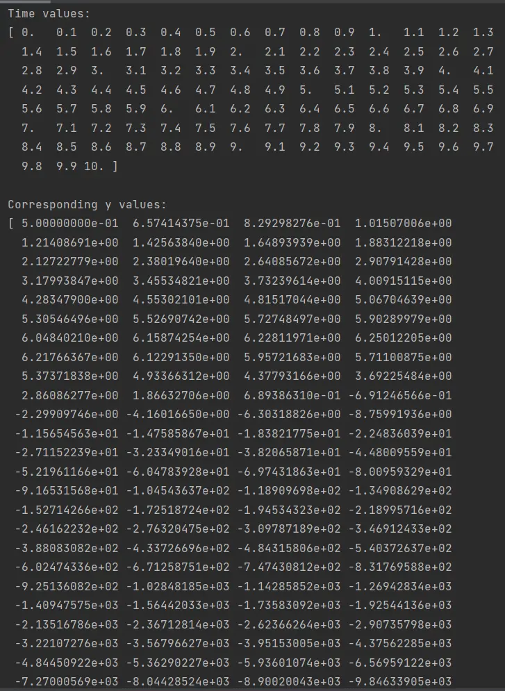
print("Time values:")
print(t_values)
print("Corresponding y values:")
print(y_values)

This code showcases a basic usage of the RK4 method to solve an ODE (dy/dt = y - t^2 + 1) over a specified time span (t_span) with a particular step size (h). The resulting time values and the corresponding solution values are then printed to the console.

Adjustments to ode_func, t_span, h, or the initial condition (y0) can solve different ODEs or alter the solution behavior based on specific requirements.

Output:

Use Scikit-Learn’s Regressor With Interpolation to Imitate the ode45() Function of MATLAB in Python

MATLAB’s ode45() is a versatile ODE solver known for its adaptability in handling differential equations. While Python’s Scikit-learn library doesn’t directly provide an equivalent, we can leverage its Regressor functionality along with interpolation techniques to mimic the behavior of ode45().

Scikit-learn’s Regressor can fit a model to the ODE solution, and interpolation techniques can be used to approximate the behavior between data points.

Scikit-learn’s regressors can approximate solutions to ODEs by learning from observed data points. Interpolation methods will approximate continuous functions between observed data points, providing a smoother representation of the solution.

Example Code:

import numpy as np
from sklearn.ensemble import RandomForestRegressor
from scipy.interpolate import interp1d

# Define the ODE function


def ode_func(t):
    return np.sin(t)  # Example ODE: dy/dt = sin(t)


# Generate training data
t_start = 0
t_end = 10
num_points = 50
num_eval_points = 100

t_train = np.linspace(t_start, t_end, num_points)
y_train = [ode_func(t) for t in t_train]

# Fit a regressor
regressor = RandomForestRegressor()
regressor.fit(t_train.reshape(-1, 1), y_train)

# Predict at evaluation time points
t_eval = np.linspace(t_start, t_end, num_eval_points)
y_pred = regressor.predict(t_eval.reshape(-1, 1))

# Interpolate for a continuous solution
interp_func = interp1d(t_eval, y_pred, kind="cubic")

# Print the exact and approximated solutions
print("Exact Solution:")
exact_solution = [ode_func(t) for t in t_eval]
print(exact_solution)

print("Approximated Solution:")
approximated_solution = interp_func(t_eval)
print(approximated_solution)

Output:

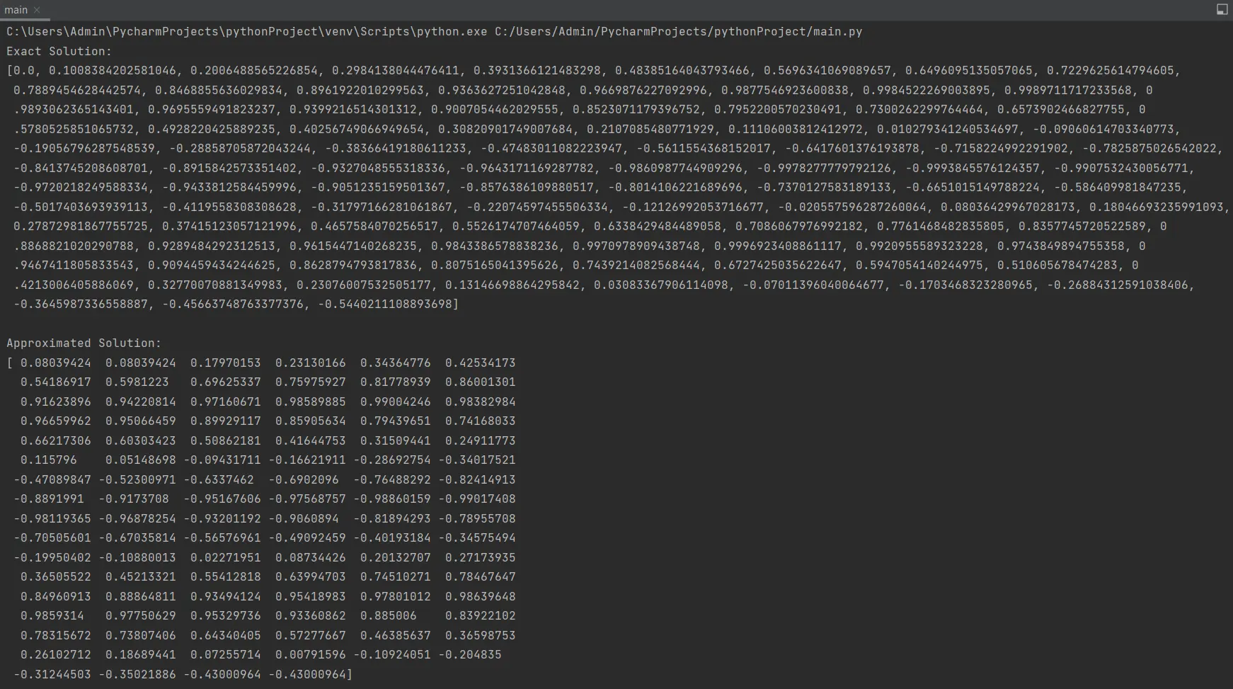
This code demonstrates how to approximate the solution of an ODE by training a regressor on generated data points and using interpolation techniques in Python. It generates training data, trains a regressor, predicts values, and performs interpolation to create a continuous function that approximates the solution of the ODE.

Adjust the ODE function, parameters, and regression method as needed for different ODEs and desired accuracy.

Conclusion

The quest to replicate the functionality of MATLAB’s ode45() function within Python showcases the versatility and adaptability of various libraries and methods in the Python ecosystem. Although there isn’t a direct equivalent, several approaches come close to emulating its behavior.

In summary, while Python doesn’t offer a direct mirror of ode45(), its versatile ecosystem empowers users with multiple approaches to solve and approximate ordinary differential equations, each with its strengths and adaptability to diverse problem domains.

Whether it’s utilizing SciPy’s comprehensive functions, implementing custom numerical schemes, or harnessing the capabilities of machine learning libraries like Scikit-learn, Python provides a rich toolkit for solving ODEs across various scientific and engineering disciplines.