Fama-Macbeth Regression in Python
- Fama-Macbeth Regression and Its Importance
- Steps to Implement the Fama-Macbeth Regression in Python
-
Use
LinearModelsto Implement the Fama-Macbeth Regression in Python - Alternative Approach to Implement the Fama-Macbeth Regression in Python

Today’s article educates about Fama-Macbeth regression, its importance, and its implementation.
Fama-Macbeth Regression and Its Importance
In asset pricing theories, we use risk factors to describe asset returns. These risk factors can be microeconomic or macroeconomic.
The microeconomic risk factors include firm size and the firm’s different financial metrics, while macroeconomic risk factors are consumer inflation and unemployment.
The Fama-Macbeth regression is a two-step regression model used to test the asset pricing models. It is a practical approach to measure how correctly these risk factors describe portfolio or asset returns.
This model is useful for determining the risk premium associated with exposure to these factors.
Now, the point is, why do we call Fama-Macbeth, a two-step regression model? Let’s find out these steps below.
- This step is about regressing every asset’s return against one or multiple risk factors using the time-series approach. We get the return exposure to every factor known as
betas,factor loadings, orfactor exposure. - This step is about regressing all assets’ returns against the asset
betasacquired in the previous step (step 1) using a cross-section approach. Here, we get a risk premium for every factor.
The projected premium over time for the unit exposure to every risk factor is then calculated by averaging coefficients once for every element, according to Fama and Macbeth.
Steps to Implement the Fama-Macbeth Regression in Python
According to the update to reflect library circumstances for Fama-Macbeth as of Fall 2018, fama_macbeth has been eradicated from the Python pandas module for a while now.
So, how can we implement Fama-Macbeth if we are working with Python? We have the following two approaches that we will learn one by one in this tutorial.
- We can use the
fama_macbethfunction inLinearModelsif we use Python version 3. - If we are not required to use
LinearModels, or we are using Python version 2, then most probably the best case would be to write our implementation for Fama-Macbeth.
Use LinearModels to Implement the Fama-Macbeth Regression in Python
-
Import the necessary modules and libraries.
import pandas as pd
import numpy as np
from pathlib import Path
from linearmodels.asset_pricing import LinearFactorModel
from statsmodels.api import OLS, add_constant
import matplotlib.pyplot as plt
import pandas_datareader.data as web
import seaborn as sns
import warnings

warnings.filterwarnings("ignore")
sns.set_style("whitegrid")
First, we import all the modules and libraries we will need to implement Fama-Macbeth using
LinearModels. A brief description of all of them is given below:- We import
pandasfor working with data frames andnumpyfor arrays. - The
pathlibmakes a path to the specified file by placing this specific script in thePathobject. - We import
LinearFactorModelfromlinearmodels.asset_pricing. The linear factor models relates the return on the asset to values of a restricted/limited number offactors, with a relationship that is described by a linear equation. - Next, we import
OLSto evaluate the linear regression model andadd_constantto add a column of ones to the array. You can learn more aboutstatsmodelshere. - After that, we import
pandas_datareaderto access the latest remote data to use withpandas. It works for variouspandasversions. - We import
matplotlibandseabornlibraries for data plotting and visualization purposes. - We import
Warningsto use itsfilterwarnings()method, which ignores warnings. - Lastly, we use the
set_style()method from theseabornmodule, which sets the parameters that control plots’ general style.
- We import
-
Access remote risk factor & research portfolio dataset.
ff_research_data_five_factor = "F-F_Research_Data_5_Factors_2x3"
ff_factor_dataset = web.DataReader(
    ff_research_data_five_factor, "famafrench", start="2010", end="2017-12"
)[0]
Here, we are using the updated risk factor & research portfolio dataset (the five Fama-French factors) available on their website to return to a monthly frequency which we get for
2010-2017as given above.We use
DataReader()to extract data from the specified internet resource into thepandasdata frame, which isff_factor_datasetin our code fence. TheDataReader()supports various sources, for instance,Tiingo,IEX,Alpha Vantage, and more that you can read on this page.print("OUTPUT for info(): \n") print(ff_factor_dataset.info())Next, we use
df.info()anddf.describe()methods whereinfo()prints the data frame’s information which includes the number of columns, data types of columns, column labels, range index, memory usage, and the number of cells in every column (non-null values).You can see the output produced by
info()below.OUTPUT:
OUTPUT for info():

<class 'pandas.core.frame.DataFrame'>
PeriodIndex: 96 entries, 2010-01 to 2017-12
Freq: M
Data columns (total 6 columns):
#   Column Non-Null Count Dtype
---  ------  --------------  -----
0   Mkt-RF 96 non-null     float64
1   SMB     96 non-null     float64
2   HML     96 non-null     float64
3   RMW     96 non-null     float64
4   CMA     96 non-null     float64
5   RF      96 non-null     float64
dtypes: float64(6)
memory usage: 5.2 KB
None
Next, we use the
describe()method as follows.print("OUTPUT for describe(): \n") print(ff_factor_dataset.describe())The
describe()method shows the data frame’s statistical summary; we can also use this method for Python series. This statistical summary contains mean, median, count, standard deviation, columns’ percentile values, and min-max.You can find the output of the
describe()method below.OUTPUT:
OUTPUT for describe(): Mkt-RF SMB HML RMW CMA RF count 96.000000 96.000000 96.000000 96.000000 96.000000 96.000000 mean 1.158438 0.060000 -0.049271 0.129896 0.047708 0.012604 std 3.580012 2.300292 2.202912 1.581930 1.413033 0.022583 min -7.890000 -4.580000 -4.700000 -3.880000 -3.240000 0.000000 25% -0.917500 -1.670000 -1.665000 -1.075000 -0.952500 0.000000 50% 1.235000 0.200000 -0.275000 0.210000 0.010000 0.000000 75% 3.197500 1.582500 1.205000 1.235000 0.930000 0.010000 max 11.350000 7.040000 8.190000 3.480000 3.690000 0.090000 -
Access 17 industry portfolios and subtract risk factor rate.
ff_industry_portfolio = "17_Industry_Portfolios"
ff_industry_portfolio_dataset = web.DataReader(
    ff_industry_portfolio, "famafrench", start="2010", end="2017-12"
)[0]
ff_industry_portfolio_dataset = ff_industry_portfolio_dataset.sub(
    ff_factor_dataset.RF, axis=0
)
Here, we use
DataReader()to access 17 industry portfolios or assets at a monthly frequency and subtract therisk-freerate (RF) from the data frame returned byDataReader(). Why? It is because the factor model works with the excess returns.Now, we will use the
info()method to get information about the chained data frame.print(ff_industry_portfolio_dataset.info())OUTPUT:
<class 'pandas.core.frame.DataFrame'>
PeriodIndex: 96 entries, 2010-01 to 2017-12
Freq: M
Data columns (total 17 columns):
#   Column Non-Null Count Dtype
---  ------  --------------  -----
0   Food    96 non-null     float64
1   Mines   96 non-null     float64
2   Oil     96 non-null     float64
3   Clths   96 non-null     float64
4   Durbl   96 non-null     float64
5   Chems   96 non-null     float64
6   Cnsum   96 non-null     float64
7   Cnstr   96 non-null     float64
8   Steel   96 non-null     float64
9   FabPr   96 non-null     float64
10 Machn   96 non-null     float64
11 Cars    96 non-null     float64
12 Trans   96 non-null     float64
13 Utils   96 non-null     float64
14 Rtail   96 non-null     float64
15 Finan   96 non-null     float64
16 Other   96 non-null     float64
dtypes: float64(17)
memory usage: 13.5 KB
None
Similarly, we describe this data frame using the
describe()method.print(ff_industry_portfolio_dataset.describe())OUTPUT:
Food Mines Oil Clths Durbl Chems \ count 96.000000 96.000000 96.000000 96.000000 96.000000 96.000000 mean 1.046771 0.202917 0.597187 1.395833 1.151458 1.305000 std 2.800555 7.904401 5.480938 5.024408 5.163951 5.594161 min -5.170000 -24.380000 -11.680000 -10.000000 -13.160000 -17.390000 25% -0.785000 -5.840000 -3.117500 -1.865000 -2.100000 -1.445000 50% 0.920000 -0.435000 0.985000 1.160000 1.225000 1.435000 75% 3.187500 5.727500 4.152500 3.857500 4.160000 4.442500 max 6.670000 21.940000 15.940000 17.190000 16.610000 18.370000 Cnsum Cnstr Steel FabPr Machn Cars \ count 96.000000 96.000000 96.000000 96.000000 96.000000 96.000000 mean 1.186979 1.735521 0.559167 1.350521 1.217708 1.279479 std 3.142989 5.243314 7.389679 4.694408 4.798098 5.719351 min -7.150000 -14.160000 -20.490000 -11.960000 -9.070000 -11.650000 25% -0.855000 -2.410000 -4.395000 -1.447500 -2.062500 -1.245000 50% 1.465000 2.175000 0.660000 1.485000 1.525000 0.635000 75% 3.302500 5.557500 4.212500 3.837500 4.580000 4.802500 max 8.260000 15.510000 21.350000 17.660000 14.750000 20.860000 Trans Utils Rtail Finan Other count 96.000000 96.000000 96.000000 96.000000 96.000000 mean 1.463750 0.896458 1.233958 1.248646 1.290938 std 4.143005 3.233107 3.512518 4.839150 3.697608 min -8.560000 -6.990000 -9.180000 -11.140000 -7.890000 25% -0.810000 -0.737500 -0.952500 -1.462500 -1.090000 50% 1.480000 1.240000 0.865000 1.910000 1.660000 75% 4.242500 2.965000 3.370000 4.100000 3.485000 max 12.980000 7.840000 12.440000 13.410000 10.770000 -
Compute the excess returns.
Before moving toward the calculation of excess returns, we have to perform a few more steps.
data_store = Path("./data/assets.h5")

wiki_prices_df = pd.read_csv(
    "./dataset/wiki_prices.csv",
    parse_dates=["date"],
    index_col=["date", "ticker"],
    infer_datetime_format=True,
).sort_index()

us_equities_data_df = pd.read_csv("./dataset/us_equities_data.csv")

with pd.HDFStore(data_store) as hdf_store:
    hdf_store.put("quandl/wiki/prices", wiki_prices_df)

with pd.HDFStore(data_store) as hdf_store:
    hdf_store.put("us_equities/stocks", us_equities_data_df.set_index("ticker"))
First, we create an
assets.h5file in adatafolder which resides in the current directory. Next, we use theread_csv()method to read thewiki_prices.csvandus_equities_data.csvfiles in thedatasetfolder from the same directory.After that, we use
HDFStore()as given above to store data inHDF5format.with pd.HDFStore("./data/assets.h5") as hdf_store: prices = hdf_store["/quandl/wiki/prices"].adj_close.unstack().loc["2010":"2017"] equities = hdf_store["/us_equities/stocks"].drop_duplicates() sectors = equities.filter(prices.columns, axis=0).sector.to_dict() prices = prices.filter(sectors.keys()).dropna(how="all", axis=1) returns_df = prices.resample("M").last().pct_change().mul(100).to_period("M") returns_df = returns.dropna(how="all").dropna(axis=1) print(returns_df.info())In the above code fence, we read the
/quandl/wiki/prices&/us_equities/stocksthat we just stored in theassets.h5file and saved them in thepricesandequitiesvariables.Then, we apply some filters on
pricesandequities, resample, and remove missing values. Finally, we print the information of a data framereturns_dfusing theinfo()method; you can see the output below.OUTPUT:
<class 'pandas.core.frame.DataFrame'>
PeriodIndex: 95 entries, 2010-02 to 2017-12
Freq: M
Columns: 1986 entries, A to ZUMZ
dtypes: float64(1986)
memory usage: 1.4 MB
None
Now, execute the following code to align the data.
ff_factor_dataset = ff_factor_dataset.loc[returns_df.index]
ff_industry_portfolio_dataset = ff_industry_portfolio_dataset.loc[returns_df.index]
print(ff_factor_dataset.describe())
OUTPUT:
		Mkt-RF        SMB        HML        RMW        CMA         RF
count 95.000000 95.000000 95.000000 95.000000 95.000000 95.000000
mean    1.206000   0.057053  -0.054316   0.144632   0.043368   0.012737
std     3.568382   2.312313   2.214041   1.583685   1.419886   0.022665
min    -7.890000  -4.580000  -4.700000  -3.880000  -3.240000   0.000000
25%    -0.565000  -1.680000  -1.670000  -0.880000  -0.965000   0.000000
50%     1.290000   0.160000  -0.310000   0.270000   0.010000   0.000000
75%     3.265000   1.605000   1.220000   1.240000   0.940000   0.010000
max    11.350000   7.040000   8.190000   3.480000   3.690000   0.090000
Now, we are ready to calculate the excess returns.
excess_returns_df = returns_df.sub(ff_factor_dataset.RF, axis=0)
excess_returns_df = excess_returns_df.clip(
    lower=np.percentile(excess_returns_df, 1),
    upper=np.percentile(excess_returns_df, 99),
)
excess_returns_df.info()
In the above code block, we subtract the risk factor from the
ff_factor_datasetand save the returned data frame inexcess_returns_df.Next, we use the
.clip()method that trims the values at the specified input threshold(s). Lastly, useinfo()to print the information of theexcess_returns_dfdata frame.OUTPUT:
<class 'pandas.core.frame.DataFrame'>
PeriodIndex: 95 entries, 2010-02 to 2017-12
Freq: M
Columns: 1986 entries, A to ZUMZ
dtypes: float64(1986)
memory usage: 1.4 MB
Before moving towards the first stage of Fama-Macbeth regression, we use the
.drop()method, which drops the specified label from columns or rows. Note thataxis=1means a drop from a column, andaxis=0means a drop from rows.ff_factor_dataset = ff_factor_dataset.drop("RF", axis=1) print(ff_factor_dataset.info())OUTPUT:
<class 'pandas.core.frame.DataFrame'> PeriodIndex: 95 entries, 2010-02 to 2017-12 Freq: M Data columns (total 5 columns): # Column Non-Null Count Dtype --- ------ -------------- ----- 0 Mkt-RF 95 non-null float64 1 SMB 95 non-null float64 2 HML 95 non-null float64 3 RMW 95 non-null float64 4 CMA 95 non-null float64 dtypes: float64(5) memory usage: 4.5 KB None -
Implement the Fama-Macbeth regression step 1: Factor Exposures.
betas = []
for industry in ff_industry_portfolio_dataset:
    step_one = OLS(
        endog=ff_industry_portfolio_dataset.loc[ff_factor_dataset.index, industry],
        exog=add_constant(ff_factor_dataset),
    ).fit()
    betas.append(step_one.params.drop("const"))

betas = pd.DataFrame(
    betas,
    columns=ff_factor_dataset.columns,
    index=ff_industry_portfolio_dataset.columns,
)
print(betas.info())
The code snippet above implements the first step of Fama-Macbeth regression and accesses the 17-factor loading estimates. Here, we use
OLS()to evaluate the linear regression model andadd_constant()to add a column of ones to the array.OUTPUT:
<class 'pandas.core.frame.DataFrame'> Index: 17 entries, Food to Other Data columns (total 5 columns): # Column Non-Null Count Dtype --- ------ -------------- ----- 0 Mkt-RF 17 non-null float64 1 SMB 17 non-null float64 2 HML 17 non-null float64 3 RMW 17 non-null float64 4 CMA 17 non-null float64 dtypes: float64(5) memory usage: 1.3+ KB None -
Implement the Fama-Macbeth regression step 2: Risk Premia.
lambdas = []
for period in ff_industry_portfolio_dataset.index:
    step_two = OLS(
        endog=ff_industry_portfolio_dataset.loc[period, betas.index], exog=betas
    ).fit()
    lambdas.append(step_two.params)

lambdas = pd.DataFrame(
    lambdas, index=ff_industry_portfolio_dataset.index, columns=betas.columns.tolist()
)
print(lambdas.info())
In the second step, we run ninety-six regressions of
periodreturns for the portfolio’s cross-section on factor loadings.OUTPUT:
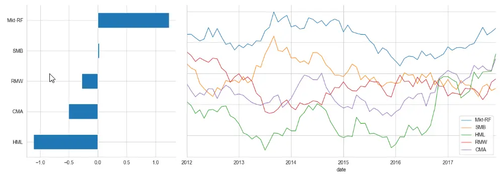
<class 'pandas.core.frame.DataFrame'>
PeriodIndex: 95 entries, 2010-02 to 2017-12
Freq: M
Data columns (total 5 columns):
#   Column Non-Null Count Dtype
---  ------  --------------  -----
0   Mkt-RF 95 non-null     float64
1   SMB     95 non-null     float64
2   HML     95 non-null     float64
3   RMW     95 non-null     float64
4   CMA     95 non-null     float64
dtypes: float64(5)
memory usage: 6.5 KB
None
We can visualize the results as follows:
window = 24  # here 24 is the number of months
axis1 = plt.subplot2grid((1, 3), (0, 0))
axis2 = plt.subplot2grid((1, 3), (0, 1), colspan=2)
lambdas.mean().sort_values().plot.barh(ax=axis1)
lambdas.rolling(window).mean().dropna().plot(
    lw=1, figsize=(14, 5), sharey=True, ax=axis2
)
sns.despine()
plt.tight_layout()
OUTPUT:
-
Implement the Fama-Macbeth regression with the
LinearModelsmodule.model = LinearFactorModel( portfolios=ff_industry_portfolio_dataset, factors=ff_factor_dataset ) result = model.fit() print(result)Here, we use the
LinearModelsto implement the two-step Fama-Macbeth procedure that produces the following output. We can useprint(result.full_summary)instead ofprint(result)to get the full summary.OUTPUT:
					LinearFactorModel Estimation Summary
================================================================================
No. Test Portfolios:                 17   R-squared:                      0.6879
No. Factors:                          5   J-statistic:                    15.619
No. Observations:                    95   P-value                         0.2093
Date:                  Mon, Oct 24 2022   Distribution:                 chi2(12)
Time:                          20:53:52
Cov. Estimator:                  robust

						  Risk Premia Estimates
==============================================================================
		  Parameter Std. Err.     T-stat    P-value    Lower CI    Upper CI
------------------------------------------------------------------------------
Mkt-RF         1.2355     0.4098     3.0152     0.0026      0.4324      2.0386
SMB            0.0214     0.8687     0.0246     0.9804     -1.6813      1.7240
HML           -1.1140     0.6213    -1.7931     0.0730     -2.3317      0.1037
RMW           -0.2768     0.8133    -0.3403     0.7336     -1.8708      1.3172
CMA           -0.5078     0.5666    -0.8962     0.3701     -1.6183      0.6027
==============================================================================

Covariance estimator:
HeteroskedasticCovariance
See full_summary for complete results
Alternative Approach to Implement the Fama-Macbeth Regression in Python
We can use this approach if we don’t want to use LinearModels or using Python version 2. For instance, it may be helpful to explore how to implement linear regression in Python. You can read more about it in our article on How to Implement Linear Regression in Python.
-
Import the modules and libraries.
import pandas as pd
import numpy as np
import statsmodels.formula.api as sm
We import
pandasto work with data frames,numpyto play with arrays, andstatsmodels.formula.api, which is a convenience interface to specify models via formula string and data frames. -
Read and query dataset.
Assume that we have Fama-French industry assets/portfolios in the panel as given below (we have also calculated a few variables, for instance, past
betaandreturnsto utilize as ourxvariables)data_df = pd.read_csv("industry_data.csv", parse_dates=["caldt"]) data_df.query("caldt == '1995-07-01'")OUTPUT:
industry caldt ret beta r12to2 r36to13 18432 Aero 1995-07-01 6.26 0.9696 0.2755 0.3466 18433 Agric 1995-07-01 3.37 1.0412 0.1260 0.0581 18434 Autos 1995-07-01 2.42 1.0274 0.0293 0.2902 18435 Banks 1995-07-01 4.82 1.4985 0.1659 0.2951 -
Use
groupby()to compute cross-sectional regression model month-by-month.def ols_coefficient(x, formula): return sm.ols(formula, data=x).fit().params gamma_df = data_df.groupby("caldt").apply( ols_coefficient, "ret ~ 1 + beta + r12to2 + r36to13" ) gamma_df.head()Here, we use
groupbybecause Fama-Macbeth involves calculating the exact cross-sectional regression model month-by-month. We can create a function that accepts a data frame (which is returned bygroupby) and apastyformula; it will then fit the model and return parameter estimates.OUTPUT:
Intercept beta r12to2 r36to13 caldt 1963-07-01 -1.497012 -0.765721 4.379128 -1.918083 1963-08-01 11.144169 -6.506291 5.961584 -2.598048 1963-09-01 -2.330966 -0.741550 10.508617 -4.377293 1963-10-01 0.441941 1.127567 5.478114 -2.057173 1963-11-01 3.380485 -4.792643 3.660940 -1.210426 -
Compute mean and standard error on mean.
def fm_summary(p):
    s = p.describe().T
    s["std_error"] = s["std"] / np.sqrt(s["count"])
    s["tstat"] = s["mean"] / s["std_error"]
    return s[["mean", "std_error", "tstat"]]


fm_summary(gamma_df)
Next, we calculate the mean, t-test (you can use any statistics you want), and standard error on the mean, which is something as above.
OUTPUT:
mean std_error tstat Intercept 0.754904 0.177291 4.258000 beta -0.012176 0.202629 -0.060092 r12to2 1.794548 0.356069 5.039896 r36to13 0.237873 0.186680 1.274230 -
Improve speed and use the
fama_macbethfunction.def ols_np(dataset, y_var, x_var): gamma_df, _, _, _ = np.linalg.lstsq(dataset[x_var], dataset[y_var], rcond=None) return pd.Series(gamma_df)This step is important if we are concerned about efficiency. If so, we can switch from
statsmodelsto thenumpy.linalg.lstsq.To perform
olsestimations, we can write a function similar to the above. Note that we are not doing anything to check these matrices’ ranks.If you are using the older
pandasversion, then the following should work. Let’s have an example using thefama_macbethinpandas.print(data_df) fm = pd.fama_macbeth(y=data_df["y"], x=data_df[["x"]]) print(fm)Here, observe the structure below. The
fama_macbethwants thex-varandy-varto have a multi-index withdateas the first variable andstock/firm/entityid as the second variable in the index.OUTPUT:
			  y    x
date       id
2012-01-01 1   0.1 0.4
		 2   0.3 0.6
		 3   0.4 0.2
		 4   0.0 1.2
2012-02-01 1   0.2 0.7
		 2   0.4 0.5
		 3   0.2 0.1
		 4   0.1 0.0
2012-03-01 1   0.4 0.8
		 2   0.6 0.1
		 3   0.7 0.6
		 4   0.4 -0.1


----------------------Summary of the Fama-Macbeth Analysis-------------------------

Formula: Y ~ x + intercept
# betas :   3

----------------------Summary of the Estimated Coefficients------------------------
   Variable          Beta       Std Err        t-stat       CI 2.5%      CI 97.5%
		(x)       -0.0227        0.1276         -0.18       -0.2728        0.2273
(intercept)        0.3531        0.0842          4.19        0.1881        0.5181

--------------------------------End of the Summary---------------------------------
Note that we are calling
fm.summaryby just printing thefmas we did in the above code fence. Additionally, thefama_macbethautomatically adds theinterceptandx-varmust be a data frame.We can do as follows if we don’t want to have
intercept.fm = pd.fama_macbeth(y=data_df["y"], x=data_df[["x"]], intercept=False)