How to Plot NumPy Linear Fit in Matplotlib Python

1. Understanding the Basics of Linear Fit
2. Creating Sample Data
3. Fitting the Linear Model
4. Plotting the Data and the Fit
5. Conclusion
6. FAQ

In the world of data science and analytics, visualizing data is crucial for understanding trends and patterns. One effective way to achieve this is by fitting a linear model to your data points and plotting it using Python’s powerful libraries, NumPy and Matplotlib. This tutorial will guide you through the process of using the numpy.polyfit() method to compute the best-fit line and how to display this line alongside your data points using Matplotlib.

Whether you are a beginner or an experienced programmer, this tutorial provides clear, step-by-step instructions to help you visualize your data effectively. By the end, you will not only have a solid understanding of how to plot a linear fit but also how to interpret the results. So, let’s dive in and start plotting!

Understanding the Basics of Linear Fit

Before we jump into the code, it’s important to understand what a linear fit is. A linear fit is a straight line that best represents the relationship between two variables in a dataset. The equation of a line is typically expressed as y = mx + b, where m is the slope and b is the y-intercept. In Python, we can easily calculate these parameters using the numpy.polyfit() function, which fits a polynomial of a specified degree to our data.

To visualize the fit, we will use Matplotlib, a popular plotting library in Python. It allows us to create a wide variety of static, animated, and interactive plots. In this article, we will focus on creating a simple linear plot with a best-fit line.

Creating Sample Data

To demonstrate how to plot a linear fit, we need some sample data. For this example, we will generate random data points that roughly follow a linear trend. Here’s how you can create this data using NumPy:

import numpy as np

# Generate random data
np.random.seed(0)
x = np.random.rand(100) * 10
y = 2.5 * x + np.random.randn(100) * 2

In this code snippet, we use np.random.seed(0) to ensure that our random data is reproducible. We then generate 100 random x-values scaled between 0 and 10. The y-values are computed based on a linear relationship with some added noise, simulating real-world data.

The generated data will be used for plotting a linear fit in the subsequent steps.

Fitting the Linear Model

Now that we have our sample data, the next step is to fit a linear model using the numpy.polyfit() method. This method returns the slope and intercept of the best-fit line. Here’s how to do it:

# Fit a linear model
slope, intercept = np.polyfit(x, y, 1)

The np.polyfit(x, y, 1) function takes three arguments: the x-values, the y-values, and the degree of the polynomial (1 for linear). It returns the slope and intercept, which we can use to plot our best-fit line.

Plotting the Data and the Fit

With the slope and intercept calculated, we can now visualize both the original data points and the fitted line using Matplotlib. Here’s the code to create the plot:

import matplotlib.pyplot as plt
import numpy as np

# Generate random data
np.random.seed(0)
x = np.random.rand(100) * 10
y = 2.5 * x + np.random.randn(100) * 2

slope, intercept = np.polyfit(x, y, 1)

# Create a scatter plot of the data
plt.scatter(x, y, color='blue', label='Data Points')

# Create the best-fit line
best_fit_line = slope * x + intercept
plt.plot(x, best_fit_line, color='red', label='Best Fit Line')

# Add labels and title
plt.xlabel('X-axis')
plt.ylabel('Y-axis')
plt.title('Linear Fit Example')
plt.legend()
plt.show()

This code snippet does several things:

1. It creates a scatter plot of the data points in blue.
2. It calculates the y-values for the best-fit line using the slope and intercept we obtained earlier.
3. It plots the best-fit line in red.
4. Finally, it adds labels, a title, and a legend before displaying the plot.

Output:

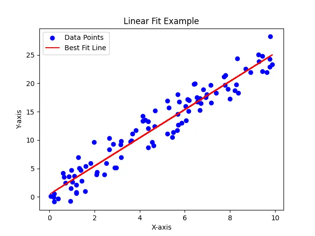
The resulting plot will clearly show how well the best-fit line represents the data points, allowing you to visually assess the linear relationship.

Conclusion

In this tutorial, we explored how to fit a linear model to data using the numpy.polyfit() method and visualize the results with Matplotlib. We started by creating sample data, fitting a linear model, and finally plotting both the data points and the best-fit line. This process is fundamental in data analysis and can be applied to various datasets to uncover trends and insights.

By mastering these techniques, you can enhance your data visualization skills and make better-informed decisions based on your analyses. Happy plotting!

FAQ

1. what is numpy.polyfit() used for?
   numpy.polyfit() is used to fit a polynomial of a specified degree to a set of data points, returning the coefficients that define the polynomial.

2. how do I visualize data in Python?
   You can visualize data in Python using Matplotlib, a powerful library that allows you to create a variety of plots and graphs.

3. can I fit polynomials of degrees higher than one?
   Yes, you can fit polynomials of any degree using numpy.polyfit() by changing the degree parameter.

4. what is the importance of data visualization?
   Data visualization helps to reveal patterns, trends, and insights in data, making it easier to understand and communicate findings.

5. how can I customize my plots in Matplotlib?
   You can customize your plots in Matplotlib by adjusting colors, labels, titles, and other parameters using various functions provided by the library.