SciPy scipy.stats.norm

1. Syntax of scipy.stats.norm() to Calculate Binomial Distribution:
2. Example Codes : Calculating Probability Distribution Function (PDF) values of Given Values Using scipy.stats.norm
3. Example Code : Calculating Cumulative Distribution Function (CDF) of Distribution Using scipy.stats.norm()
4. Example Codes : Calculating Random variates (rvs) of Distribution Using scipy.stats.norm()

Python Scipy scipy.stats.norm object is used to analyze the normal distribution and calculate its different distribution function values using the different methods available.

Syntax of scipy.stats.norm() to Calculate Binomial Distribution:

Based on different methods used, some common optimal parameters are shown below:

scipy.stats.norm.method(x, loc, scale, size, moments)

Methods Available in scipy.stats.norm() Object

Parameters

Return

It returns values as per the methods used.

Example Codes : Calculating Probability Distribution Function (PDF) values of Given Values Using scipy.stats.norm

We can use the scipy.stats.norm.pdf() method to generate the Probability Distribution Function (PDF) value of the given observations.

import numpy as np
import matplotlib.pyplot as plt
import scipy
from scipy import stats

x = np.linspace(-3, 3, 100)
pdf_result = stats.norm.pdf(x, loc=0, scale=1)

plt.plot(x, pdf_result)
plt.xlabel("x-data")
plt.ylabel("pdf_value")
plt.title("PDF of a Normal Distribution with mean=0 and sigma=1")
plt.show()

Output:

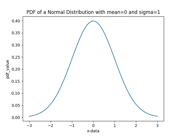
Suppose x represents the values of observation whose PDF is to be determined. Now we calculate the Probability Distribution Function(PDF) of each value in the x, and plot the distribution function using Matplotlib.

To calculate the Probability Density Function value, we must know the mean and standard deviation of the underlying normal distribution. The values of mean and standard deviation are passed as loc and scale parameters in the pdf method, respectively.

In the above example, we calculate pdf values assuming underlying distribution has a mean value of 0 and standard deviation value of 1. The observations near the mean have a higher probability. On the other hand, the values away from the mean have less probability, as seen in the plot above.

Example Codes : Set mean and standard deviation values in scipy.stats.norm

import numpy as np
import matplotlib.pyplot as plt
import scipy
from scipy import stats

x = np.linspace(-10, 10, 100)
pdf_result = stats.norm.pdf(x, loc=3, scale=2)

plt.plot(x, pdf_result)
plt.xlabel("x-data")
plt.ylabel("pdf_value")
plt.title("PDF of a Normal Distribution with mean=3 and sigma=2")
plt.show()

Output:

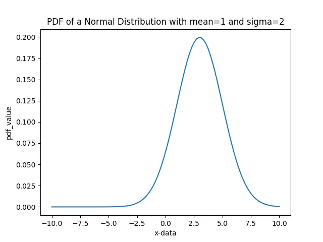
It is the PDF plot of a normal distribution with mean value 3 and sigma value 2. Hence, observations near 3 have a higher probability, while those away from 3 have a lesser probability.

Example Code : Calculating Cumulative Distribution Function (CDF) of Distribution Using scipy.stats.norm()

import numpy as np
import matplotlib.pyplot as plt
import scipy
from scipy import stats

x = np.linspace(-3, 3, 100)
cdf_values = stats.norm.cdf(x, loc=0, scale=1)

plt.plot(x, cdf_values)
plt.xlabel("x-data")
plt.ylabel("pdf_value")
plt.title("CDF of a Normal Distribution with mean=0 and sigma=1")
plt.show()

Output:

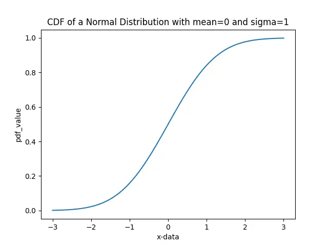
It is the integral of pdf. We can see that the CDF of the given distribution is increasing. CDF shows us that any value taken from the population will have a probability value less than or equal to some value.

Example Code : Calculating Cumulative Distribution Function (CDF) value at a Point Using scipy.stats.norm()

import numpy as np
import matplotlib.pyplot as plt
import scipy
from scipy import stats

x = 2
cdf_value = stats.norm.cdf(x, loc=0, scale=1)
print(
    "CDF Value of x=2 in normal distribution with mean 0 and standard deviation 1 is :"
    + str(cdf_value)
)

Output:

CDF Value of x=2 in normal distribution with mean 0 and standard deviation 1 is :0.9772498680518208.

It implies the probability of occurrence of value less than or equal to 2 while sampling from a normal distribution with mean=0 and standard deviation 1 is:0.977.

Example Codes : Calculating Random variates (rvs) of Distribution Using scipy.stats.norm()

import numpy as np
import matplotlib.pyplot as plt
import scipy
from scipy.stats import norm

rvs_values = stats.norm.rvs(loc=5, scale=10, size=(5, 2))
print("The random generated value are\n", rvs_values)

Output:

The random generated value are
 [[ -8.38511257  16.81403567]
 [ 15.78217954  -8.92401338]
 [ 14.55202276  -0.6388562 ]
 [  2.19024898   3.75648045]
 [-10.95451165  -3.98232268]]

Here, rvs values are the randomly generated variates sampled from the normal distribution with mean 5 and standard deviation 10. The size specifies the size of the array output.