SciPy scipy.stats.multivariate_normal

Python Scipy scipy.stats.multivariate_normal object is used to analyze the multivariate normal distribution and calculate different parameters related to the distribution using the different methods available.

Syntax to Gemerate Probability Density Function Using scipy.stats.multivariate_normal Object

scipy.stats.multivariate_normal.pdf(x, mean=None, cov=1, allow_singular=False)

Parameters:

Return:

An array-like structure which contains probability value for each element in x.

Example : Generate Probability Density Function Using scipy.stats.multivariate_normal.pdf Method

import numpy as np
from scipy.stats import multivariate_normal

mean = np.array([0.4, 0.8])
cov = np.array([[0.1, 0.3], [0.3, 1.0]])
x = np.random.uniform(size=(5, 2))
y = multivariate_normal.pdf(x, mean=mean, cov=cov)

print("Tha data and corresponding pdfs are:")
print("Data-------PDF value")
for i in range(len(x)):
    print(x[i], end=" ")
    print("------->", end=" ")
    print(y[i], end="\n")

Output:

Tha data and corresponding pdfs are:
Data-------PDF value
[0.60156002 0.53917659] -------> 0.030687330659191728
[0.60307471 0.25205368] -------> 0.0016016741361277501
[0.27254519 0.06817383] -------> 0.7968146411119688
[0.33630808 0.21039553] -------> 0.7048988855032084
[0.0009666  0.52414497] -------> 0.010307396714783708

In the above example, x represents the array of values whose pdf is to be found. The rows represent each value of x whose pdf is to be found, and columns represent the number of components used to represent each value.

Here, each value of x consists of two components, and hence it is a vector of length 2. The mean will be a vector with a length equal to the number of components. Similarly, if d be the number of components in the dataset, cov will be a symmetric square matrix of size d*d.

The scipy.stats.multivariate_normal.pdf method takes the input x, mean and covariance matrix cov and outputs a vector with a length equal to the number of rows in x where each value in the output vector represents pdf value for each row in x.

Example : Draw Random Samples From a Multivariate Normal Distribution Using scipy.stats.multivariate_normal.rvs Method

import numpy as np
import matplotlib.pyplot as plt
from scipy.stats import multivariate_normal

mean = np.array([0.4, 0.8])
cov = np.array([[0.1, 0.3], [0.3, 1.0]])
x = multivariate_normal.rvs(mean, cov, 100)
plt.scatter(x[:, 0], x[:, 1])
plt.show()

Output:

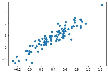
The above plot represents the scatter plot of 20 random samples drawn randomly from a multivariate normal distribution with two features. The distribution has mean value of [0.4,0.8] where 0.4 represents the mean value of the first feature and 0.8 the mean of the second feature. We finally draw the scatter plot of random samples with the first feature along the X-axis and the second feature along the Y-axis.

From the plot, it is clear that most of the sample points are centered around [0.4,0.8], representing the multivariate distribution’s mean.

Example : Get Cumulative Distribution Function Using scipy.stats.multivariate_normal.cdf Method

Cumulative distribution function (CDF) is the integral of pdf.CDF shows us that any value taken from the population will have a probability value less than or equal to some value. We can calculate cdf of points of multivariate distribution using the scipy.stats.multivariate_normal.cdf method.

import numpy as np
from scipy.stats import multivariate_normal

mean = np.array([0.4, 0.8])
cov = np.array([[0.1, 0.3], [0.3, 1.0]])
x = np.random.uniform(size=(5, 2))
y = multivariate_normal.cdf(x, mean=mean, cov=cov)

print("Tha data and corresponding cdfs are:")
print("Data-------CDF value")
for i in range(len(x)):
    print(x[i], end=" ")
    print("------->", end=" ")
    print(y[i], end="\n")

Output:

Tha data and corresponding cdfs are:
Data-------CDF value
[0.89027577 0.06036432] -------> 0.22976054289355996
[0.78164237 0.09611703] -------> 0.24075282906929418
[0.53051197 0.63041372] -------> 0.4309184323329717
[0.15571201 0.97173575] -------> 0.21985053519541042
[0.72988545 0.22477096] -------> 0.28256819625802715

In the above example, x represents the array of points at which cdf is to be found. The rows represent each value of x at which cdf is to be found, and columns represent the number of components used to represent each value.

Here, each value of x consists of two components, and hence it is a vector of length 2. The mean will be a vector with a length equal to the number of components. Similarly, if d be the number of components in the dataset, cov will be a symmetric square matrix of size d*d.

The scipy.stats.multivariate_normal.cdf method takes the input x, mean and covariance matrix cov and outputs a vector with a length equal to the number of rows in x where each value in the output vector represents cdf value for each row in x.