Bilinear Interpolation in Python

1. Create a User-Defined Function to Implement Bilinear Interpolation in Python
2. Use the scipy.interpolate.interp2d() to Implement Bilinear Interpolation in Python
3. Use the scipy.interpolate.RectBivariateSpline() to Implement Bilinear Interpolation in Python
4. Conclusion

Bilinear interpolation is a method used to estimate values between two known values. This technique is commonly employed in computer graphics, image processing, and geometric transformations.

In this article, we’ll explore how to implement bilinear interpolation in Python.

Create a User-Defined Function to Implement Bilinear Interpolation in Python

Bilinear interpolation is particularly useful when you have a grid of values and need to estimate the value at a non-grid point. It involves calculating the weighted average of the four nearest grid points to approximate the value at an arbitrary point within the grid.

In the context of a rectangular grid, we can represent four neighboring points as (a1, b1), (a1, b2), (a2, b1), and (a2, b2). The values at these points are denoted as x11, x12, x21, and x22, respectively.

The goal is to interpolate the value at coordinates (a, b) within this grid. Let’s discuss the process of implementing bilinear interpolation in Python.

Sorting Points

The first step involves sorting the input points based on their coordinates. The four points representing the corners of the rectangle are sorted to ensure consistent ordering, which simplifies subsequent calculations.

sorted_pts = sorted(pts)
(a1, b1, x11), (_a1, b2, x12), (a2, _b1, x21), (_a2, _b2, x22) = sorted_pts

Here, sorted_pts contains the sorted list of four points, and we unpack them into variables (a1, b1, x11), (_a1, b2, x12), (a2, _b1, x21), (_a2, _b2, x22).

Checking Rectangle Validity

We then check whether the sorted points form a valid rectangle. We verify that the x and y coordinates of the corners are consistent with the expected rectangle structure.

if a1 != _a1 or a2 != _a2 or b1 != _b1 or b2 != _b2:
    print("The given points do not form a rectangle")

If the points don’t meet the rectangle criteria, a warning is printed.

Checking Point Validity

Next, we check whether the input coordinates (a, b) are within the bounds of the rectangle. If they are not, a warning is printed.

if not a1 <= a <= a2 or not b1 <= b <= b2:
    print("The (a, b) coordinates are not within the rectangle")

Bilinear Interpolation Formula

The core of the function implements the bilinear interpolation formula, which calculates the weighted average of the four surrounding points based on their distances from the target coordinates (a, b).

Y = (
    x11 * (a2 - a) * (b2 - b)
    + x21 * (a - a1) * (b2 - b)
    + x12 * (a2 - a) * (b - b1)
    + x22 * (a - a1) * (b - b1)
) / ((a2 - a1) * (b2 - b1) + 0.0)

The formula involves multiplying the value at each corner by a set of weightings based on the relative distances of the target coordinates to the corners. The result is divided by the total area of the rectangle.

Finally, we return the calculated value Y, which represents the result of the bilinear interpolation for the given coordinates (a, b) within the specified rectangle. We can then use this result as needed for further computations or visualization.

Complete Code Example

Here’s the complete Python function bilinterpol:

def bilinterpol(a, b, pts):
    sorted_pts = sorted(pts)
    (a1, b1, x11), (_a1, b2, x12), (a2, _b1, x21), (_a2, _b2, x22) = sorted_pts

    if a1 != _a1 or a2 != _a2 or b1 != _b1 or b2 != _b2:
        print("The given points do not form a rectangle")

    if not a1 <= a <= a2 or not b1 <= b <= b2:
        print("The (a, b) coordinates are not within the rectangle")

    Y = (
        x11 * (a2 - a) * (b2 - b)
        + x21 * (a - a1) * (b2 - b)
        + x12 * (a2 - a) * (b - b1)
        + x22 * (a - a1) * (b - b1)
    ) / ((a2 - a1) * (b2 - b1) + 0.0)

    return Y


pts = [
    (0, 1, 12),
    (4, 1, 0),
    (0, 3, -4),
    (4, 3, 8),
]

# Test the function with coordinates (2, 3)
result = bilinterpol(2, 3, pts)
print(result)

Now, let’s demonstrate how to use our bilinterpol function with a set of sample points.

2.0

In this example, the function is applied to the coordinates (2, 3) using the provided points. The expected output is 2.0, representing the estimated value at the given non-grid point.

Use the scipy.interpolate.interp2d() to Implement Bilinear Interpolation in Python

The scipy.interpolate.interp2d() function is part of the SciPy library, which is widely used for scientific and technical computing in Python. Specifically, this function is designed for 2D interpolation, making it suitable for scenarios where you have a grid of data points and need to estimate values at non-grid points.

Here’s the syntax of the scipy.interpolate.interp2d() function:

scipy.interpolate.interp2d(
    x, y, z, kind="linear", copy=True, bounds_error=False, fill_value=None
)

Parameters:

• x and y: Arrays representing the data points’ coordinates. x denotes the column coordinates, while y represents the row coordinates on the grid.
• z: Array-like values specifying the function’s values corresponding to the given set of data points.
• kind: Specifies the type of interpolation to be used. Options include linear, cubic, or quintic. The default is linear.
• copy: If True, the input arrays are copied. If False, the function may modify the input arrays.
• bounds_error: If True, an error is raised for out-of-bounds interpolation points. If False, values outside the input range are assigned fill_value.
• fill_value: Value used to fill in for points outside the convex hull of the input points.

Before diving into code, it’s crucial to understand the data you’re working with. Bilinear interpolation assumes that your data is on a 2D grid, where each point has corresponding x, y, and z values.

Importing Necessary Libraries

Import the required libraries, including scipy.interpolate for the interpolation function, numpy for array operations, and matplotlib.pyplot for visualization.

from scipy import interpolate
import numpy as np
import matplotlib.pyplot as plt

Generating Sample Data

Create a set of sample data points. This involves defining x and y coordinates and generating corresponding function values (z) on a 2D grid.

In this example, we use the numpy.arange() and numpy.meshgrid() functions for this purpose.

x = np.arange(-15.01, 15.01, 1.00)
y = np.arange(-15.01, 15.01, 1.00)
xx, yy = np.meshgrid(x, y)
z = np.cos(xx**2 + yy**2)

Creating the Interpolation Function

Use the scipy.interpolate.interp2d() function to create an interpolation function. Specify the kind of interpolation you want (linear, cubic, quintic, etc.).

f = interpolate.interp2d(x, y, z, kind="quintic")

In this case, we choose "quintic" for smoother results.

Generating New Coordinates for Interpolation

Create a set of new coordinates where you want to interpolate values. These coordinates should be within the range of your original data.

xnew = np.arange(-15.01, 15.01, 1e-2)
ynew = np.arange(-15.01, 15.01, 1e-2)

Performing Interpolation

Apply the interpolation function to the new coordinates to obtain interpolated values. The result is a set of z values corresponding to the new coordinates.

znew = f(xnew, ynew)

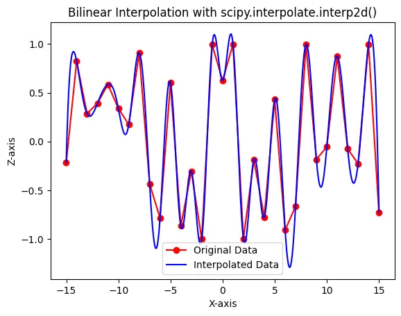
Visualizing the Results

Use matplotlib.pyplot to create a plot comparing the original data with the interpolated data. Visualization is crucial for understanding the effectiveness of the interpolation.

plt.plot(x, z[0, :], "ro-", label="Original Data")
plt.plot(xnew, znew[0, :], "b-", label="Interpolated Data")
plt.legend()
plt.title("Bilinear Interpolation with scipy.interpolate.interp2d()")
plt.xlabel("X-axis")
plt.ylabel("Z-axis")
plt.show()

Now, let’s put these steps into action with a practical example:

from scipy import interpolate
import numpy as np
import matplotlib.pyplot as plt

x = np.arange(-15.01, 15.01, 1.00)
y = np.arange(-15.01, 15.01, 1.00)
xx, yy = np.meshgrid(x, y)
z = np.cos(xx**2 + yy**2)

f = interpolate.interp2d(x, y, z, kind="quintic")

xnew = np.arange(-15.01, 15.01, 1e-2)
ynew = np.arange(-15.01, 15.01, 1e-2)

znew = f(xnew, ynew)

plt.plot(x, z[0, :], "ro-", label="Original Data")
plt.plot(xnew, znew[0, :], "b-", label="Interpolated Data")
plt.legend()
plt.title("Bilinear Interpolation with scipy.interpolate.interp2d()")
plt.xlabel("X-axis")
plt.ylabel("Z-axis")
plt.show()

Output:

Use the scipy.interpolate.RectBivariateSpline() to Implement Bilinear Interpolation in Python

Note that the interp2d() function is deprecated in SciPy 1.10, and it will be removed in SciPy 1.13.0. To address this, we can use the RectBivariateSpline class as a replacement for regular grids.

The RectBivariateSpline() class in SciPy is designed for spline interpolation on a rectangular grid. It provides a flexible and efficient way to perform bilinear interpolation for regularly spaced data.

Syntax:

scipy.interpolate.RectBivariateSpline(x, y, z, kx=3, ky=3)

Parameters:

• x, y: 1-D arrays representing the coordinates of the grid.
• z: 2-D array representing the values of the function at the grid points.
• kx, ky: The order of the spline interpolation along the x and y directions. Adjust based on the desired level of smoothness.

Let’s go through the steps to implement bilinear interpolation using RectBivariateSpline:

Import Necessary Libraries

Import the required libraries, including scipy.interpolate.RectBivariateSpline, numpy for array operations, and matplotlib.pyplot for visualization.

from scipy.interpolate import RectBivariateSpline
import numpy as np
import matplotlib.pyplot as plt

Generating Sample Data

Create a set of sample data points. Define x and y coordinates and generate corresponding function values (z) on a 2D grid.

x = np.arange(-15.01, 15.01, 1.00)
y = np.arange(-15.01, 15.01, 1.00)
xx, yy = np.meshgrid(x, y)
z = np.cos(xx**2 + yy**2)

Creating the Interpolation Function

Use the RectBivariateSpline class to create an interpolation function. Adjust the kx and ky parameters based on the desired smoothness.

f = RectBivariateSpline(x, y, z, kx=3, ky=3)

Generating New Coordinates for Interpolation

Create a set of new coordinates where you want to interpolate values. These coordinates should be within the range of your original data.

xnew = np.arange(-15.01, 15.01, 1e-2)
ynew = np.arange(-15.01, 15.01, 1e-2)

Performing Interpolation

Apply the interpolation function to the new coordinates to obtain interpolated values.

znew = f(xnew, ynew)

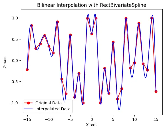
Visualizing the Results

Use matplotlib.pyplot to create a plot comparing the original data with the interpolated data.

plt.plot(x, z[0, :], "ro-", label="Original Data")
plt.plot(xnew, znew[0, :], "b-", label="Interpolated Data")
plt.legend()
plt.title("Bilinear Interpolation with RectBivariateSpline")
plt.xlabel("X-axis")
plt.ylabel("Z-axis")
plt.show()

We basically did the same process as with the interp2d() function.

Complete Code Example

Here’s the complete code:

from scipy.interpolate import RectBivariateSpline
import numpy as np
import matplotlib.pyplot as plt

x = np.arange(-15.01, 15.01, 1.00)
y = np.arange(-15.01, 15.01, 1.00)
xx, yy = np.meshgrid(x, y)
z = np.cos(xx**2 + yy**2)

f = RectBivariateSpline(x, y, z, kx=3, ky=3)  # Adjust kx and ky as needed

xnew = np.arange(-15.01, 15.01, 1e-2)
ynew = np.arange(-15.01, 15.01, 1e-2)

znew = f(xnew, ynew)

plt.plot(x, z[0, :], "ro-", label="Original Data")
plt.plot(xnew, znew[0, :], "b-", label="Interpolated Data")
plt.legend()
plt.title("Bilinear Interpolation with RectBivariateSpline")
plt.xlabel("X-axis")
plt.ylabel("Z-axis")
plt.show()

Output:

In this modified code, RectBivariateSpline is used instead of interp2d. The parameters kx and ky control the order of the spline interpolation along the x and y directions, respectively.

Adjust them based on your specific requirements.

Conclusion

In conclusion, this article has provided a thorough exploration of bilinear interpolation in Python, offering three distinct methods for implementation. The user-defined function approach allows for a detailed understanding of the interpolation process, involving sorting points, checking validity, and applying the interpolation formula.

On the other hand, the use of the RectBivariateSpline class from SciPy provides a powerful and efficient alternative, particularly as the interp2d() function is deprecated. Whether opting for a customized solution or leveraging library functionality, mastering bilinear interpolation is a valuable skill for tasks involving grid-based data interpolation and analysis in Python.