MATLAB kstest() Function

This tutorial will discuss finding the test decision of the null hypothesis for a data set used to check if a data set is from a standard normal distribution or if it does not come from a standard normal distribution using the kstest() function in MATLAB.

Matlab kstest() Function

In Matlab, the kstest() function is used to find the test decision of the null hypothesis for a data set which is used to check if a data set is from a standard normal distribution or if it does not come from a standard normal distribution. The kstest() function uses the one sample Kolmogorov Smirnov algorithm to find the test decision.

The basic syntax of the kstest() function is below.

output = kstest(data)

The output of the above syntax can be 0 or 1. If the output is 0, the function does not reject the test decision for the null hypothesis, and if the output is 1, it means the function has rejected the test decision.

Let’s discuss an example of exam grades to confirm the test decision of the kstest() function. We can plot the standard normal distribution and the empirical cumulative distribution on a single plot to compare them and confirm the test decision.

See the example code and output below.

clc
clear

load examgrades
data = grades(:,1);
a = (data-75)/10;
testResult = kstest(a)

cdfplot(a)
hold on
x = linspace(min(a),max(a));
plot(x,normcdf(x,0,1),'r--')
legend('Empirical-CDF','Normal-CDF')

Output:

testResult =

  logical

   0

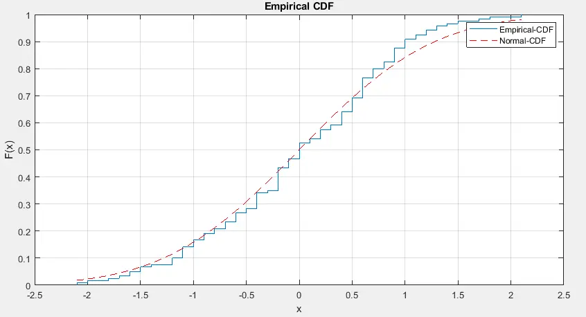
We have used the examgrades data set, which is already in Matlab in the above code. We have used a mean of 75 and a standard deviation of 10 to make the data set from the given grades, and we passed it inside the kstest() function, which returned 0 as the test decision value, which means the function has not rejected the test decision of the null hypothesis.

If we look at the output picture above, we can see that the two distributions are close to each other, which confirms that the test decision is accurate. We have used the cdfplot() function to plot the cumulative distribution function of the data and the normcdf() function to find the normal distribution of the given data.

We have used the legend() function to add legends to the plot to understand it easily. Now, let’s change the mean from 75 to 85 in the above code and check the result.

See the example code and output below.

clc
clear

load examgrades
data = grades(:,1);
a = (data-85)/10;
testResult = kstest(a)

cdfplot(a)
hold on
x = linspace(min(a),max(a));
plot(x,normcdf(x,0,1),'r--')
legend('Empirical-CDF','Normal-CDF')

Output:

testResult =

  logical

   1

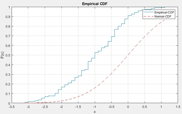
In the above code, the kstest() function has returned 1, which means the test decision is rejected, and we can also confirm it using the above picture, which clearly shows the two distributions and not equal to each other.

We can also specify the hypothesized distribution while finding the test decision using the two-column matrix. The first column contains the data and the second column contains the cumulative distribution values or cdf.

We also have to tell the kstest() function about it using the CDF argument, as shown below.

output = kstest(data,'CDF',cdfOfData)

In the above code, the cdfOfData is a two-column matrix in which the first column is the data and the second column is the cdf of that data. We can find cdf using Matlab’s cdf() function.

We can also specify the hypothesized distribution using a probability distribution object which we can make using the makedist() function. Check this link for more details about the makedist() function.

We have to pass the distribution object inside the kstest() function using the CDF argument, as shown below.

output = kstest(data,'CDF',cdfObject)

We can also find the test decision on different significant levels using the Alpha argument and setting its value from 0 to 1. The kstest() function will also return a new argument, p, which shows the probability of a test decision.

An example of the kstest() function with the Alpha argument is shown below.

[output, p] = kstest(data,'CDF',cdfObject, 'Alpha', 0.2)

We can also check the test decision using an alternate hypothesis using the Tail argument in which the kstest() function will return 0 or 1 in favor of the alternate hypothesis. The value of the Tail argument can be unequal, larger, or smaller.

By default, the value of the Tail argument is set to unequal, meaning the cdf of the population and the cdf of the hypothesized distribution will not be equal. The larger value sets the cdf of the population greater than the cdf of the hypothesized distribution, and the smaller value sets the population cdf less than the hypothesized cdf.

An example of the kstest() function with the Tail argument is shown below.

output = kstest(data, 'Tail', 'larger')

The kstest() function returns four total arguments shown in the syntax below.

[h,p,ksstat,cv] = kstest(data)

We are already familiar with the first two arguments of the kstest() function.

The ksstat argument contains nonnegative scaler values of the statistic of the hypothesis test. The cv argument has the critical value, a nonnegative scalar.

Matlab also contains the kstest2() function, which is used to test the decision of two vectors using the two sample Kolmogorov Smirnov algorithm.

Check this link for more details about the kstest() function.