How to Apply Geometric Transformation to Images in MATLAB

This tutorial will discuss applying the geometric transformation to an image using the imwarp() function in MATLAB.

Apply Geometric Transformation to Images in MATLAB

Geometric transformation transforms images according to our requirements like rotating, resizing, and shearing images. We can use the imwarp() function in MATLAB to apply a geometric transform to an image.

An image consists of pixels placed in specific locations. The imwrap() function changes the location of pixels according to the given transformation object.

For example, if we want to flip an image vertically, we only have to change the position of the pixels present in the image. The top row of pixels will be interchanged with the last row of pixels present in the given image.

The basic syntax of the imwarp() function is given below.

output_image = imwarp(input_image, geo_tran);

We can use the above syntax to apply a given geometric transform geo_tran to an input image input_image, and the result will be stored inside the output_image. The input image can be a numeric, logical, or categorical image.

We can create a 2D geometric transformation object or matrix using the affine2d() function of MATLAB. We have to define a 3-by-3 matrix inside the affine2d() function to create the transformation object and pass it inside the imwarp() function to apply it to the given image.

For example, let’s use the camera image already stored in MATLAB and apply a geometric transform using the imwarp() function.

See the code below.

clc

Img = imread('cameraman.tif');
imshow(Img)
gform = affine2d([1 0 0; .5 1 0; 1 0 1])
Jmg = imwarp(Img,gform);
figure
imshow(Jmg)

Output:

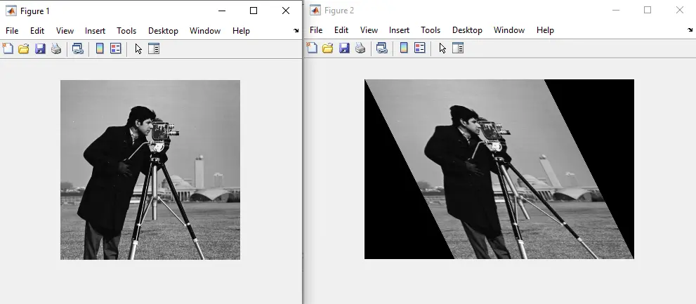
In the above output, we can see that the right side image is changed, and the only change is in the location of the pixels. We can also change the transformation matrix according to the given image and the type of output we want to get from the function.

Check this link for more details about the affine2d() function. If we want to create a geometric transformation matrix for a 3d image, we can use the affine3d() function of MATLAB.

In case of affine3d(), the input matrix should be of size 4-by-4. Check this link for more details about the affine3d() function.

Rotate an Image by N Degrees

To rotate an image, we can use the randomaffine2d() function to create a randomized 2D affine transformation object and then pass it along with the given image inside the imwarp() function to apply the transformation to the given image. We can use the Rotation argument of the randomaffine2d() function, and after that, we have to set the angle or range of the angle to create a transformation to rotate the given image.

For example, let’s rotate the above image by 45 degrees. See the code below.

clc

Img = imread('cameraman.tif');
imshow(Img)
gform = randomAffine2d('Rotation',[45 45]);
Jmg = imwarp(Img,gform);
figure
imshow(Jmg)

Output:

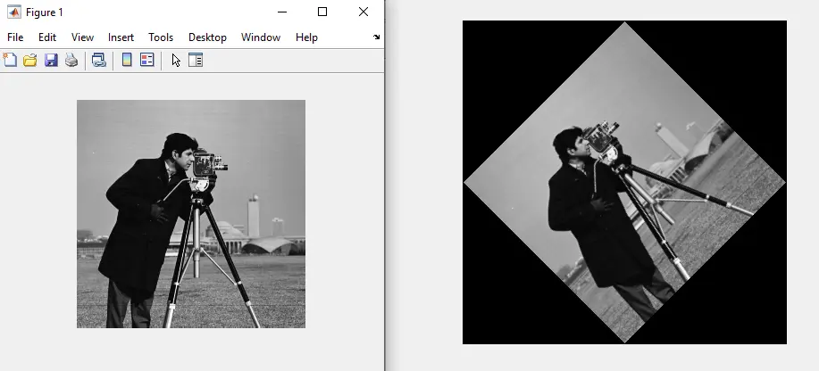
In the above code, we applied the same value of 45 twice, but we can also provide a range, and the function will pick a random angle from the range to create the transformation object.

Reflect, Scale, Shear, and Translate an Image

To create the x or y-axis reflection of the image, we can use the XReflection and YReflection arguments. After defining the argument name, we have to pass true because, by default, these arguments are set to false.

The reflection argument will flip the image horizontally or vertically. We can also shear an image which means moving one part of the image in one direction and the other part in the opposite direction.

We can also apply x or y-axis shear using the XShear and YShear arguments, and after that, we have to set the value as a 2-element vector. We can also scale the image using the scale argument of the randomaffine2d() function.

If the scale value is less than 1, the image size will decrease; if it is greater than 1, it will increase. We can also translate an image on the x or y-axis using the XTranslation and YTranslation arguments, and after that, we have to define the 2-element matrix for translation.

For example, let’s change the properties mentioned above and see the result. See the code below.

clc
clear

Img = imread('cameraman.tif');
imshow(Img)
gform = randomAffine2d('XReflection',true,'Scale',[1.2 1.2],'XShear',[15 15],'XTranslation',[20 20]);
Jmg = imwarp(Img,gform);
figure
imshow(Jmg)

Output:

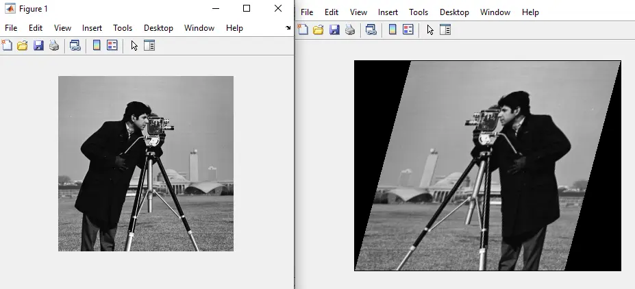
We can change each property separately to see its result on the original image. Check this link for more details about the randomaffine2d() function.

In the case of a 3D image, we can use the randomaffine3d() function to create a 3d transformation object, and we can change its properties in the same way we changed the properties of the randomaffine2d() function. Check this link for more details about the randomaffine3d() function.

Set Edges, View, and Bounding Style of the Output Image

We can also alter the properties of the imwarp() function like the interpolation method, which is set to nearest by default, and we can change it to linear or cubic. In some cases, the edges of the output image are not smooth, but we can use the SmoothEdges argument inside the imwarp() function to get smooth edges.

We can also change the output view of the output image using the OutputView argument, and after that, we have to pass a view object created using the affineOutputView() function. The first argument of the affineOutputView() function is the size of the input image, and the second argument is the transformation object.

The third optional argument, BoundingStyle, is used to set the bounding style of the output image. There are three types of styles available CenterOutput, FollowOutput, and SameAsInput style.

For example, let’s change the properties of the imwarp() function mentioned above. See the code below.

clc
clear

Img = imread('cameraman.tif');
imshow(Img)
gform = randomAffine2d('Rotation',[45 45]);
Output_view = affineOutputView(size(Img),gform,'BoundsStyle','CenterOutput');
Jmg = imwarp(Img,gform,'SmoothEdges',true,'OutputView',Output_view);
figure
imshow(Jmg)

Output:

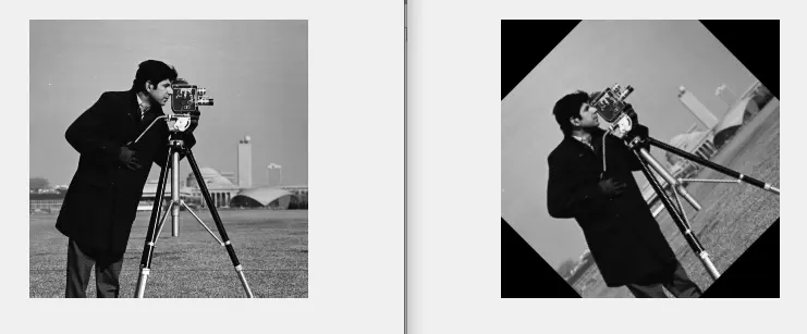
The right image (output image) has the same size as the input image because we have used the smooth edges argument. If we don’t use the smooth edges argument, the size of the output image will increase, which is also shown in the first example of rotation of the image.

Check this link for more details about the affineOutputView() function. Check this link for more details about the imwarp() function.