How to Plot CDF Matplotlib Python

This tutorial explains how we can generate a CDF plot using the Matplotlib in Python. CDF is the function whose y-values represent the probability that a random variable will take the values smaller than or equal to the corresponding x-value.

Plot CDF Using Matplotlib in Python

CDF is defined for both continuous and discrete probability distributions. In continuous probability distribution, the random variable can take any value from the specified range, but in the discrete probability distribution, we can only have a specified set of values.

Plot CDF for Discrete Distribution Using Matplotlib in Python

import numpy as np
import matplotlib.pyplot as plt

x = np.arange(1, 7)
y = [0.2, 0.1, 0.1, 0.2, 0.1, 0.3]
cdf = np.cumsum(y)

plt.plot(x, y, marker="o", label="PMF")
plt.plot(x, cdf, marker="o", label="CDF")
plt.xlim(0, 7)
plt.ylim(0, 1.5)
plt.xlabel("X")
plt.ylabel("Probability Values")
plt.title("CDF for discrete distribution")
plt.legend()
plt.show()

Output:

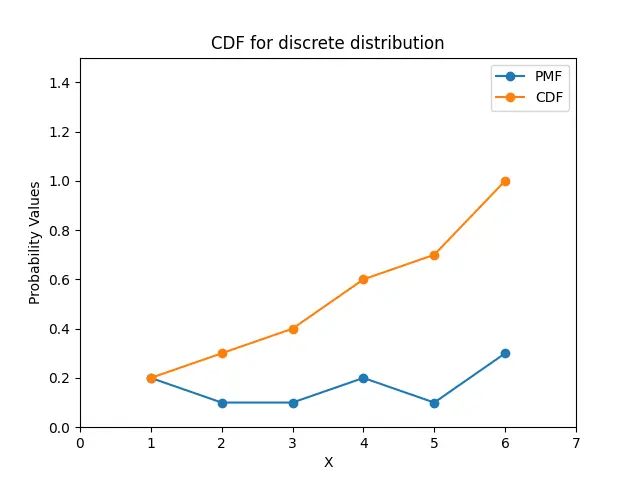
It plots the PMF and CDF for the given distribution. To calculate the y-values for CDF, we use the numpy.cumsum() method to calculate an array’s cumulative sum.

If we are given frequency counts, we must normalize the y-values initially so that they represent the PDF.

import numpy as np
import matplotlib.pyplot as plt

x = np.arange(1, 7)
frequency = np.array([3, 8, 4, 5, 3, 6])
pdf = frequency / np.sum(frequency)
cdf = np.cumsum(pdf)

plt.plot(x, pdf, marker="o", label="PMF")
plt.plot(x, cdf, marker="o", label="CDF")
plt.xlim(0, 7)
plt.ylim(0, 1.5)
plt.xlabel("X")
plt.ylabel("Probability Values")
plt.title("CDF for discrete distribution")
plt.legend()
plt.show()

Output:

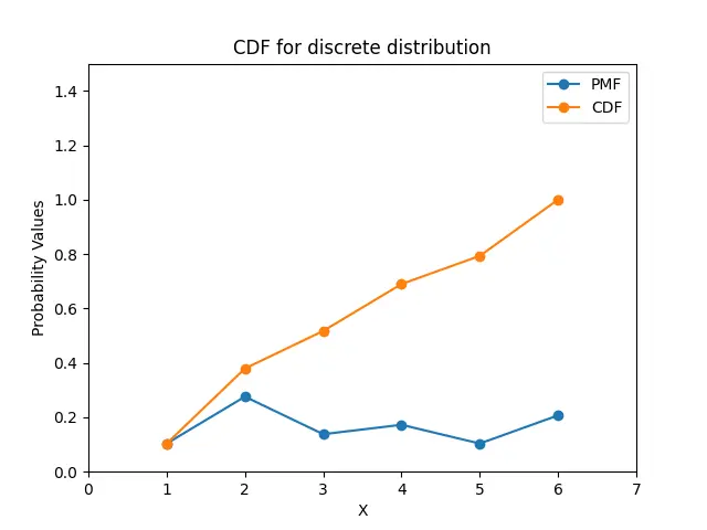
Here, we are given the frequency values for each X value. We convert the frequency values into pdf values by dividing each element of the pdf array by the sum of frequencies. We then use the pdf to calculate the CDF values to plot the CDF of given data.

We can also use histogram plots to view the CDF and PDF plots, which will be more intuitive for discrete data.

import numpy as np
import matplotlib.pyplot as plt

data = [3, 4, 2, 3, 4, 5, 4, 7, 8, 5, 4, 6, 2, 1, 0, 9, 7, 6, 6, 5, 4]
plt.hist(data, bins=9, density=True)
plt.hist(data, bins=9, density=True, cumulative=True, label="CDF", histtype="step")
plt.xlabel("X")
plt.ylabel("Probability")
plt.xticks(np.arange(0, 10))
plt.title("CDF using Histogram Plot")
plt.show()

Output:

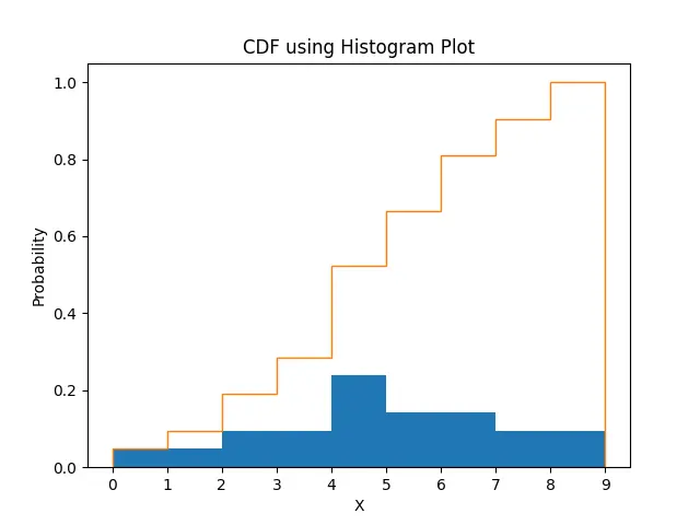
It plots the CDF and PDF of given data using the hist() method. To plot the CDF, we set cumulative=True and set density=True to get a histogram representing probability values that sum to 1.

Plot CDF for Continuous Distribution Using Matplotlib in Python

import numpy as np
import matplotlib.pyplot as plt

dx = 0.005
x = np.arange(-10, 10, dx)
y = 0.25 * np.exp((-(x ** 2)) / 8)

y = y / (np.sum(dx * y))
cdf = np.cumsum(y * dx)

plt.plot(x, y, label="pdf")
plt.plot(x, cdf, label="cdf")
plt.xlabel("X")
plt.ylabel("Probability Values")
plt.title("CDF for continuous distribution")
plt.legend()
plt.show()

Output:

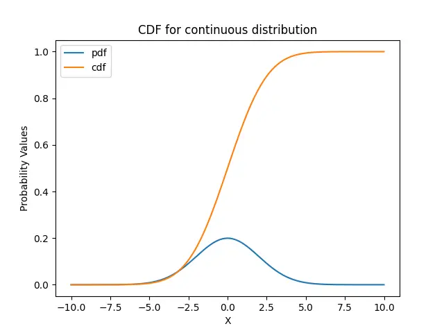
It plots the PMF and CDF for the given continuous distribution. To calculate the y-values for CDF, we use the numpy.cumsum() method to calculate an array’s cumulative sum.

We divide y by the sum of the array y multiplied by the dx to normalize the values so that the CDF values range from 0 to 1.