MATLAB fzero Function

This tutorial will discuss finding the roots of a nonlinear function using the fzero() function in MATLAB.

MATLAB fzero() Function

The fzero() function is used to find the roots of a nonlinear function. The function uses different interpolation methods like secant and bisection methods to find the roots of the given nonlinear function.

The basic syntax of the fzero() function is below.

roots = fzero(fun, x0);

The above syntax will return the roots of the fun starting from the point x0. For example, let’s find the value of pi by finding the roots of the sine function near 3.

See the code below.

clc
clear

f = @sin;
x0 = 3;
value = fzero(f,x0)

Output:

value = 3.1416

The clc and clear commands are used to clear the command and the workspace window in the above code. As we can see in the output, the value returned by the fzero() function is approximately equal to the value of pi.

Instead of passing a single point as the starting point, we can also pass an interval to find the root of the given nonlinear function. For example, let’s find the root of the cosine function in the interval of 1 to 3.

See the code below.

clc
clear

f = @cos;
x0 = [1 3];
value = fzero(f,x0)

Output:

value = 1.5708

Note that the values of the function at the endpoints of the interval should differ in sign; otherwise, there will be an error, and if the error appears, we have to change the sign of one of the interval values. We did not use interval values with different signs in the above code because cos(1) and cos(3) signs already differ.

Note that the input function whose root we want to find should have one parameter only, and if it has more than one parameter, we have to pass the values of the other parameters before finding the root. For example, let’s create a function with two parameters, pass the value of one parameter, and then find the root of the function.

See the code below.

clc
clear

f = @(x,c) cos(c*x);
c = 3;
f_1 = @(x) f(x,c);
x = fzero(f_1,0.1)

Output:

x = 0.5236

In the above output, we passed the f_1 function inside the fzero() function because the f function contains two parameters, and its root will not be evaluated unless we pass the value of one parameter.

We can also set some other options inside the fzero() function as the plot of the current point or function value using the PlotFcns argument, setting tolerance value which by default is set to 2.2e-16 using the TolX argument, output functions which will be called at each iteration of the fzero() function using the OutputFcn argument, check the value of the objective function using the FunValCheck argument, and the level of the display using the Display argument.

To set the options, we have to make a structure of all the options using the optimset() function. For example, let’s set the above options for a nonlinear function.

See the code below.

clc
clear

f = @(x,c) cos(c*x);
c = 3;
f_1 = @(x) f(x,c);
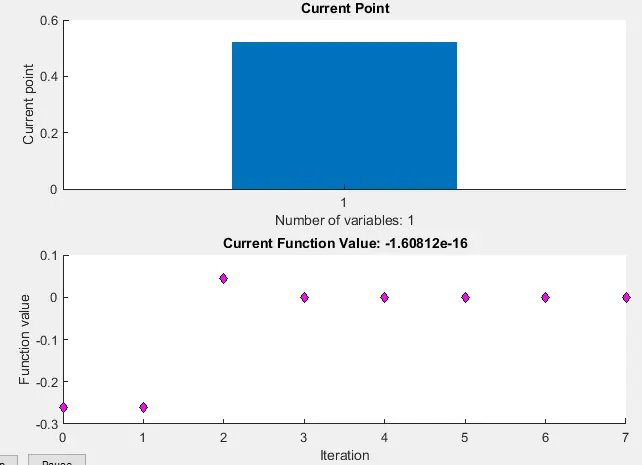
options = optimset('PlotFcns',{@optimplotx,@optimplotfval},'Display','final','FunValCheck','on','TolX',1.1e-16);
x = fzero(f_1,0.1,options)

Output:

Zero found in the interval [-0.412, 0.612]

x = 0.5236

In the above output, we can see the interval where zero has been found, and we can also see the plot of the current point and the plot of function values at different iterations.

The display option has four types off for no output, iter for output at each iteration, final for only final output, and notify for output only if the function does not converge.

We can set the FunValCheck option to on or off, and if it is set to on, the function will display an error if the output is infinity, NaN, or complex, and if it is set to off, there will be no error displayed.

We can also find the root of a function by defining it as a problem structure using the problem argument.

We will use the problem.objective command to define the function. We will use the problem.x0 command to initialize the starting point or interval.

We will use the problem.solver command to define the solving method. We can use the problem.options command to set the options.

The name problem can change to any character or string. For example, let’s use the problem structure to find the root of a nonlinear function.

See the code below.

clc
clear

p.objective = @(x)sin(cosh(x));
p.x0 = 1;
p.solver = 'fzero';
p.options = optimset(@fzero);
root = fzero(p)

Output:

root =

    1.8115

We can also get other information from the fzero() function like the function value, the exit flag, which will indicate the exit condition, and the information about the process of root finding.

The exit flag can return 1 (which indicates the function converged), -1 (which indicates the algorithm was terminated due to the output or plot function), -3 (which indicates infinity or NaN value was encountered), -4 (which indicates a complex value was encountered), -5 (which indicates algorithm converged to a singular point), and -6 (which indicates the function did not detect a change in the sign).

For example, let’s find the root of a nonlinear function and get all the information about the process. See the code below.

clc
clear

Myfun = @(x) exp(-exp(-x)) - x;
x0 = [0 1];
[root fval exitflag output] = fzero(Myfun,x0)

Output:

root =

    0.5671


fval =

     0


exitflag =

     1


output =

  struct with fields:

    intervaliterations: 0
            iterations: 5
             funcCount: 7
             algorithm: 'bisection, interpolation'
               message: 'Zero found in the interval [0, 1]'

The function also returned the interval between the iterations, total number of iterations, and algorithm used to find the root of the nonlinear function. Check this link for more details about the fzero() function.