Scipy scipy.optimize.curve_fit Method

1. Syntax of scipy.optimize.curve_fit():
2. Example Codes : scipy.optimize.curve_fit() Method to Fit Straight Line to Our Data (linear model expression)
3. Example Code : scipy.optimize.curve_fit() Method to Fit Exponential Curve to Our Data (exponential model expression)

Python Scipy scipy.optimize.curve_fit() function is used to find the best-fit parameters using a least-squares fit. The curve_fit method fits our model to the data.

The curve fit is essential to find the optimal set of parameters for the defined function that best fits the provided set of observations.

Syntax of scipy.optimize.curve_fit():

scipy.optimize.curve_fit(f, xdata, ydata, sigma=None, p0=None)

Parameters

Return

It returns two values :

1. popt : Array-like. It contains optimal values for the model function. Internally contains fit results for the slope and fit results for intercept.
2. p-cov : Covariance, which denotes uncertainties in the fit result.

Example Codes : scipy.optimize.curve_fit() Method to Fit Straight Line to Our Data (linear model expression)

import numpy as np
import matplotlib.pyplot as plt
import scipy
from scipy import optimize


def function(x, a, b):
    return a * x + b


x = np.linspace(start=-50, stop=10, num=40)
y = function(x, 6, 2)

np.random.seed(6)
noise = 20 * np.random.normal(size=y.size)
y = y + noise

popt, cov = scipy.optimize.curve_fit(function, x, y)
a, b = popt

x_new_value = np.arange(min(x), 30, 5)
y_new_value = function(x_new_value, a, b)

plt.scatter(x, y, color="green")
plt.plot(x_new_value, y_new_value, color="red")
plt.xlabel("X")
plt.ylabel("Y")
print("Estimated value of a : " + str(a))
print("Estimated value of b : " + str(b))
plt.show()

Output:

Estimated value of a : 5.859050240780936
Estimated value of b : 1.172416121927438

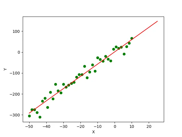
In this example, we first generate a dataset with 40 points using the y = 6*x+2 equation. Then we add some Gaussian noise to the dataset’s y values to make it look more realistic. Now we estimate the parameters a and b of the underlying equation y=a*x+b, which generates the dataset using the scipy.optimize.curve_fit() method. The green points in the plot represent the actual data points of the dataset, and the red line represents the curve fitted to the dataset using the scipy.optimize.curve_fit() method.

Finally, we can see the values of a and b estimated using the scipy.optimize.curve_fit() method are 5.859 and 1.172 respectively, which are pretty close to actual values 6 and 2.

Example Code : scipy.optimize.curve_fit() Method to Fit Exponential Curve to Our Data (exponential model expression)

import numpy as np
import matplotlib.pyplot as plt
import scipy
from scipy import optimize


def function(x, a, b):
    return a * np.exp(b * x)


x = np.linspace(10, 30, 40)

y = function(x, 0.5, 0.3)
print(y)

noise = 100 * np.random.normal(size=y.size)
y = y + noise
print(y)
popt, cov = scipy.optimize.curve_fit(function, x, y)

a, b = popt

x_new_value = np.arange(min(x), max(x), 1)
y_new_value = function(x_new_value, a, b)

plt.scatter(x, y, color="green")
plt.plot(x_new_value, y_new_value, color="red")
plt.xlabel("X")
plt.ylabel("Y")
print("Estimated value of a : " + str(a))
print("Estimated value of b : " + str(b))
plt.show()

Output:

Estimated value of a : 0.5109620054206334
Estimated value of b : 0.2997005016319089

In this example, we first generate a dataset with 40 points using the equation y = 0.5*x^0.3. Then we add some Gaussian noise to the dataset’s y values to make it more realistic. Now we estimate the parameters a and b of the underlying equation y = a*x^b which generates the dataset using the scipy.optimize.curve_fit() method. The green points in the plot represent the actual data points of the dataset, and the red line represents the curve fitted to the dataset using the scipy.optimize.curve_fit() method.

Finally, we can see the values of a and b estimated using the scipy.optimize.curve_fit() method are 0.5109 and 0.299 respectively, which are pretty close to actual values 0.5 and 0.3.

In this way, we can determine the underlying equation of given data points using the scipy.optimize.curve_fit() method.