How to Use the Sobel Operator for Image Edge Detection in MATLAB

We will look at different ways to use the Sobel method of edge detection image processing in MATLAB. We will use different example codes and related outputs to clear your concepts and give you a complete insight into the Sobel method of edge detection image processing technique in MATLAB.

Please note that edge detection encompasses a range of analytic approaches to find boundaries and contours in a computerized picture where the imagery intensity varies abruptly or, rather precisely, contains discontinuities.

Step detection identifies discontinuity in one-dimensional signals, while change detection identifies signal irregularities.

Edge detection is a powerful technique in visual analysis, machine vision, and object recognition, notably in object recognition and separation. Sobel, Canny, Prewitt, Roberts, and Fuzzy logic approaches are prominent edge detection techniques.

Use the Sobel Operator From Scratch for Image Edge Detection in MATLAB

The Sobel operator, also known as the Sobel–Feldman operator or Sobel filter, can be employed in the picture and video processing, most notably in edge detection techniques. It generates an image that emphasizes edges.

It was named in honor of Stanford Artificial Intelligence Laboratory collaborators Irwin Sobel and Gary Feldman (SAIL). In 1968, Sobel & Feldman introduced the concept of an Isotropic 3x3 Image Gradient Operator at SAIL.

A discrete differentiation operator computes an approximate gradient of the picture intensity curve. The Sobel–Feldman operation produces the matching gradient vector or the normal of this vector at every location in the picture.

The Sobel–Feldman operator is predicated on convolving the picture in the horizontal and vertical directions with a tiny, separable, integer-valued filter and is thus computationally cheap. However, the gradient approximation generated is extremely poor, especially for high-frequency fluctuations in the picture.

Let us understand this concept by looking at the following example.

Example code:

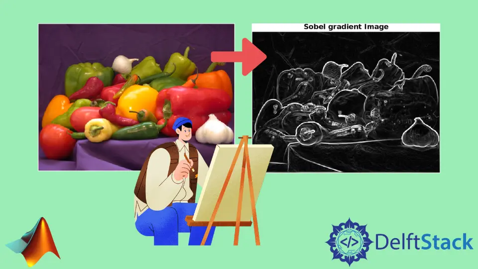
Aimage=imread('peppers.png');
imshow(Aimage)
Bimage=rgb2gray(Aimage);

Cimage=double(Bimage);

for k=1:size(Cimage,1)-2
for l=1:size(Cimage,2)-2
%Sobel mask for x-direction:
G_x=((2*Cimage(k+2,l+1)+Cimage(k+2,l)+Cimage(k+2,l+2))-(2*Cimage(k,l+1)+Cimage(k,l)+Cimage(k,l+2)));
%Sobel mask for y-direction:
G_y=((2*Cimage(k+1,l+2)+Cimage(k,l+2)+Cimage(k+2,l+2))-(2*Cimage(k+1,l)+Cimage(k,l)+Cimage(k+2,l)));
%The gradient of the image
%B(i,j)=abs(Gx)+abs(Gy);
Bimage(k,l)=sqrt(G_x.^2+G_y.^2);
end
end
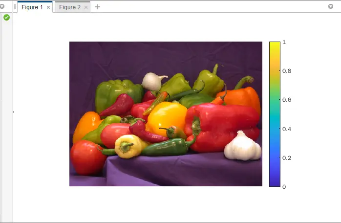
figure,
imshow(Bimage);
title('Sobel gradient Image');

Output:

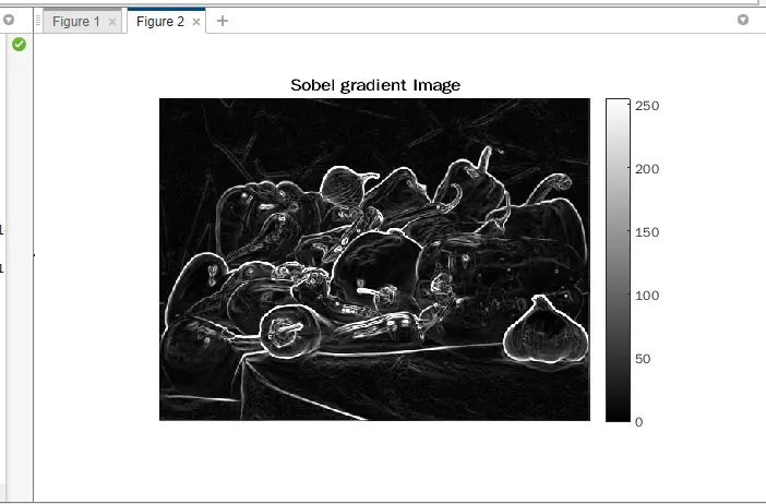
The edge detected image may be obtained from the Sobel gradient utilizing a cutoff/threshold setting. Instead, the threshold level is applied if the Sobel gradient proportions are less than the criterion level.

If f is equal to the critical threshold, f equals the predefined cutoff.

Example code:

Aimage=imread('peppers.png');
imshow(Aimage)
Bimage=rgb2gray(Aimage);

Cimage=double(Bimage);

for k=1:size(Cimage,1)-2
for l=1:size(Cimage,2)-2
%Sobel mask for x-direction:
G_x=((2*Cimage(k+2,l+1)+Cimage(k+2,l)+Cimage(k+2,l+2))-(2*Cimage(k,l+1)+Cimage(k,l)+Cimage(k,l+2)));
%Sobel mask for y-direction:
G_y=((2*Cimage(k+1,l+2)+Cimage(k,l+2)+Cimage(k+2,l+2))-(2*Cimage(k+1,l)+Cimage(k,l)+Cimage(k+2,l)));
%The gradient of the image
%B(i,j)=abs(Gx)+abs(Gy);
Bimage(k,l)=sqrt(G_x.^2+G_y.^2);
end
end
figure,
imshow(Bimage);
title('Sobel gradient Image');

%Define a threshold value
Thresholdd=100;
Bimage=max(Bimage,Thresholdd);
Bimage(Bimage==round(Thresholdd))=0;

Bimage=uint8(Bimage);
figure,
imshow(Bimage);
title('Edge detected Image');

Here, the question arises why we subtracted 2 in the i=1:size (C,1) -2 and j=1:size (C,2) -2. This is because a 3x3 frame is produced from every (i,j)th location.

By removing 2, we can keep the number inside its boundaries. That boundary results from the convolution of the Sobel 3x3 horizontal mask with the image matrix assuming we’re looking at the element C(i,j) from the source picture matrix.

To get the corresponding component in the Gx matrix, Gx(i,j), we pick the 8 neighbors around the elements C(i,j) and C(i,j), multiply each of them by the corresponding element of the Sobel mask, and add the results: C(i-1,j-1) * S(1,1)+C(i-1,j) * S(1,2) * C(i-1,j+1) * S(1,3)+.. (9 multiplications here).

Output: