플롯 결정 경계 Python
그림, 그래프 및 플롯이 포함된 결과의 시각적 요약은 인간의 마음이 주어진 데이터의 패턴을 처리, 이해 및 인식하는 데 보다 여유로운 시간을 제공합니다. 이 기사에서는 Matplotlib의 pyplot을 사용하여 결정 경계를 그리는 단계별 절차를 살펴봅니다.
이를 위해 Sklearn 라이브러리에서 제공하는 사전 처리된 내장 데이터(누락된 데이터 또는 이상값 없음) 데이터 세트 패키지를 사용하여 데이터에 대한 결정 경계를 그립니다. 그런 다음 Matplotlib의 라이브러리를 사용하여 결정 경계를 그립니다.
필수 라이브러리 설치
Matplotlib의 pyplot의 플로팅 기능을 사용하려면 먼저 Matplotlib의 라이브러리를 설치해야 합니다. 다음 명령을 실행하여 이를 달성할 수 있습니다.
pip install matplotlib
올바른 Python 버전으로 작업하는지 확인하는 것도 중요합니다. 이 문서에서는 버전 3.10.4를 사용하고 있습니다.
다음 명령을 실행하여 현재 설치된 Python 버전을 확인할 수 있습니다.
python --version
결정 경계
분류 기계 학습 알고리즘은 입력 예제(관찰)에 레이블을 할당하는 방법을 학습합니다. 분류의 목표는 레이블이 기능 공간의 점에 가능한 한 정확하게 지정되도록 기능 공간을 분리하는 것입니다.
이 방법을 의사 결정 표면 또는 경계라고 하며 분류 예측 모델의 결과를 시각화하는 실증 도구로 작동합니다. 최소 두 개의 입력 기능에 대해 선형 결정 경계를 만들 수 있습니다.
그러나 두 개 이상의 입력 기능이 있는 경우 다중 선형 결정 경계를 만들 수 있습니다. 이 문서에서는 두 입력 기능의 결정 경계를 플로팅하는 데 중점을 둘 것입니다.
Matplotlib의 pyplot을 사용하여 2개 클래스를 구분하는 결정 경계 그리기
필요한 라이브러리 가져오기
import numpy as np
import pandas as pd
import matplotlib.pyplot as plt
from matplotlib.colors import ListedColormap
from sklearn import datasets
from sklearn.linear_model import LogisticRegression
from sklearn.preprocessing import StandardScaler
from sklearn.metrics import accuracy_score, confusion_matrix
from sklearn.model_selection import train_test_split
데이터 세트 생성
datasets 클래스 내에서 Sklearn 라이브러리 make_blobs() 함수를 사용하여 사용자 지정 데이터 세트를 생성합니다. 위에서 언급했듯이 우리가 사용할 생성된 데이터 세트는 Sklearn 라이브러리에서 제공하는 사전 처리된 내장 데이터(누락된 데이터나 이상값이 없는) 데이터 세트 패키지입니다.
사용자 정의 생성 데이터 세트 변수는 다음과 같습니다.
    samples     features    standard deviation
    1000        2           3
XFeature, yFeature = datasets.make_blobs(
    n_samples=1000, centers=2, n_features=2, random_state=1, cluster_std=3
)
데이터 생성이 완료되면 데이터의 산점도를 만들어 훨씬 개선된 조명에서 데이터 변동성을 확인할 수 있습니다.
for c_value in range(2):
    row = np.where(yFeature == c_value)
    plt.scatter(XFeature[row, 0], XFeature[row, 1])
plt.show()
다음 단계에서는 보이지 않는 데이터를 예측하는 분류 모델을 구축합니다. 사용자 지정 데이터 세트에는 두 가지 기능만 있으므로 로지스틱 회귀를 사용할 수 있습니다.
로지스틱 회귀 모델
sklearn 라이브러리의 Logistic Regression 클래스에서 제공하는 Logistic Regression 모델 기능을 사용하고 샘플 데이터에 대해 학습합니다.
regressor = LogisticRegression()
regressor.fit(XFeature, yFeature)
y_pred = regressor.predict(XFeature)
이제 sklearn 라이브러리의 Accuracy_score 클래스로 정확도를 평가합니다.
accuracy = accuracy_score(y, y_pred)
print("Model Accuracy: %.3f" % accuracy)
결정 경계 생성
Matplotlib은 contour()라는 유용한 기능을 제공하는데, 이 기능은 서로 다른 점 사이를 플로팅하는 동안 색상을 추가하는 데 도움이 됩니다. 이를 달성하려면 먼저 기능 공간에서 Xfeature 또는 YFeature 포인트 그리드를 초기화해야 합니다.
그런 다음 각 기능의 최대값과 최소값을 찾은 다음 전체 공간이 포함되도록 1씩 늘려야 합니다.
min1, max1 = XFeature[:, 0].min() - 1, XFeature[:, 0].max() + 1
min2, max2 = XFeature[:, 1].min() - 1, XFeature[:, 1].max() + 1
numpy 라이브러리는 좌표를 0.1 해상도로 스케일링하는 arrange() 함수를 제공합니다.
x1_scale = np.arange(min1, max1, 0.1)
x2_scale = np.arange(min2, max2, 0.1)
다음 단계에서 numpy 라이브러리는 스케일된 좌표를 그리드로 변환하는 meshgrid() 함수를 제공합니다.
x_grid, y_grid = np.meshgrid(x1_scale, x2_scale)
그런 다음 numpy 라이브러리에서 제공하는 flatten() 함수를 사용하여 2D 배열 그리드를 1D 배열로 줄입니다.
x_g, y_g = x_grid.flatten(), y_grid.flatten()
x_g, y_g = x_g.reshape((len(x_g), 1)), y_g.reshape((len(y_g), 1))
마지막으로 1차원 배열을 입력 데이터 세트의 열로 나란히 쌓지만 훨씬 더 높은 해상도로 쌓을 것입니다.
grid = np.hstack((x_g, y_g))
그런 다음 이를 위에서 생성한 회귀 모델에 적용하여 값을 예측할 수 있습니다.
y_pred_2 = regressor.predict(grid)  # predict the probability
# keep just the probabilities for class 0
p_pred = regressor.predict_proba(grid)
p_pred = p_pred[:, 0]  # reshaping the results
p_pred.shape
pp_grid = p_pred.reshape(x_grid.shape)
이제 다양한 색상을 사용하여 contour()를 사용하여 예측된 그리드를 등고선 플롯으로 플로팅합니다.
surface = plt.contourf(x_grid, y_grid, pp_grid, cmap="Pastel1")
plt.colorbar(surface)  # create scatter plot for samples from each class
for class_value in range(2):
    row_ix = np.where(y == class_value)
    plt.scatter(X[row_ix, 0], X[row_ix, 1], cmap="Pastel1")
plt.show()
따라서 두 클래스를 구분하는 결정 경계를 그리는 다음 스크립트로 끝납니다.
전체 코드:
import numpy as np
import pandas as pd
import matplotlib.pyplot as plt
from matplotlib.colors import ListedColormap
from sklearn import datasets
from sklearn.linear_model import LogisticRegression
from sklearn.preprocessing import StandardScaler
from sklearn.metrics import accuracy_score, confusion_matrix
from sklearn.model_selection import train_test_split

XFeature, yFeature = datasets.make_blobs(
    n_samples=1000, centers=2, n_features=2, random_state=1, cluster_std=3
)

for c_val in range(2):
    row = np.where(yFeature == c_val)
    plt.scatter(XFeature[row, 0], XFeature[row, 1])
plt.show()

reg = LogisticRegression()
reg.fit(XFeature, yFeature)
y_pred = reg.predict(XFeature)

acc = accuracy_score(yFeature, y_pred)
print("Accuracy: %.3f" % acc)

min1, max1 = XFeature[:, 0].min() - 1, XFeature[:, 0].max() + 1
min2, max2 = XFeature[:, 1].min() - 1, XFeature[:, 1].max() + 1

x1_scale = np.arange(min1, max1, 0.1)
x2_scale = np.arange(min2, max2, 0.1)

x_grid, y_grid = np.meshgrid(x1_scale, x2_scale)

x_g, y_g = x_grid.flatten(), y_grid.flatten()
x_g, y_g = x_g.reshape((len(x_g), 1)), y_g.reshape((len(y_g), 1))

grid = np.hstack((x_g, y_g))

y_pred_2 = reg.predict(grid)
p_pred = reg.predict_proba(grid)
p_pred = p_pred[:, 0]
pp_grid = p_pred.reshape(x_grid.shape)

surface = plt.contourf(x_grid, y_grid, pp_grid, cmap="Pastel1")
plt.colorbar(surface)
for class_value in range(2):
    row_ix = np.where(yFeature == class_value)
    plt.scatter(XFeature[row_ix, 0], XFeature[row_ix, 1], cmap="Pastel1")
plt.show()
출력:
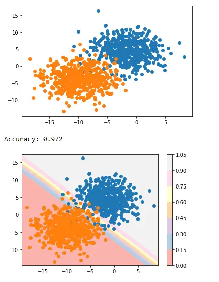
이것은 Matplotlib의 pyplot을 사용하여 두 클래스를 구분하는 결정 경계를 적용하는 방법입니다.

I am Fariba Laiq from Pakistan. An android app developer, technical content writer, and coding instructor. Writing has always been one of my passions. I love to learn, implement and convey my knowledge to others.
LinkedIn