在 Python 中執行影象分割
在本教程中,我們將學習如何使用 scikit-image 庫在 Python 中執行影象分割。
影象分割將影象分成許多層,每一層都由一個智慧的畫素級掩碼錶示。根據影象的整合級別組合、阻止和拆分影象。
在 Python 中安裝 scikit-image 模組
pip install scikit-image
安裝完成後,我們將轉換影象格式進行分割。
在 Python 中轉換影象格式
應用過濾器和其他處理技術所需的輸入是二維向量,即單色影象。
我們將使用 skimage.color.rgb2gray() 函式將 RGB 影象轉換為灰度格式。
from skimage import data, io, filters
from skimage.color import rgb2gray
import matplotlib.pyplot as plt

image = data.coffee()
plt.figure(figsize=(15, 15))
gray_coffee = rgb2gray(image)
plt.subplot(1, 2, 2)
plt.imshow(gray_coffee, cmap="gray")
plt.show()
我們在上面的程式碼中將 scikit 庫中的示例咖啡影象轉換為灰度。
讓我們看一下影象的灰度版本。

我們將使用兩種技術進行分割,即監督和無監督分割。
Python 中的監督分割
這種形式的分割需要外部輸入才能起作用。我們將使用兩種方法執行此型別。
閾值分割——Python 中的手動輸入
使用 0-255 的外部畫素值來區分影象和背景。結果,影象被更改為大於或小於給定閾值。
我們將使用以下程式碼執行此方法。
from skimage import data
from skimage import filters
from skimage.color import rgb2gray
import matplotlib.pyplot as plt
coffee = data.coffee()
gray_coffee = rgb2gray(coffee)
plt.figure(figsize=(15, 15))
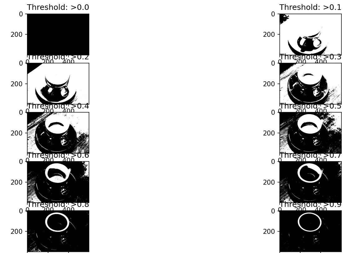
for i in range(10):
binarized_gray = (gray_coffee > i * 0.1) * 1
plt.subplot(5, 2, i + 1)
plt.title("Threshold: >" + str(round(i * 0.1, 1)))
plt.imshow(binarized_gray, cmap="gray")
plt.show()
plt.tight_layout()
現在讓我們看看上面程式碼的輸出,我們可以看到使用各種閾值分割的影象。
讓我們學習另一種稱為主動輪廓分割的監督分割方法。
Python 中的主動輪廓分割
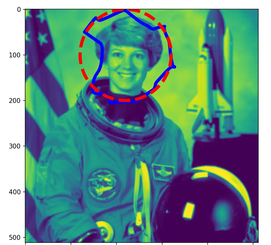
活動輪廓是一種分割方法,可將感興趣的畫素與影象的其餘部分分開,以便使用能量力和限制進行進一步處理和分析。通過將蛇擬合到影象特徵,skimage.segmentation.active_contour() 函式建立活動輪廓。
我們將使用以下程式碼來應用此方法。
import numpy as np
import matplotlib.pyplot as plt
from skimage.color import rgb2gray
from skimage import data
from skimage.filters import gaussian
from skimage.segmentation import active_contour

astronaut = data.astronaut()
gray_astronaut = rgb2gray(astronaut)
gray_astronaut_noiseless = gaussian(gray_astronaut, 1)
x1 = 220 + 100 * np.cos(np.linspace(0, 2 * np.pi, 500))
x2 = 100 + 100 * np.sin(np.linspace(0, 2 * np.pi, 500))

snake = np.array([x1, x2]).T
astronaut_snake = active_contour(gray_astronaut_noiseless, snake)

fig = plt.figure(figsize=(10, 10))
ax = fig.add_subplot(111)

ax.imshow(gray_astronaut_noiseless)

ax.plot(astronaut_snake[:, 0], astronaut_snake[:, 1], "-b", lw=5)
ax.plot(snake[:, 0], snake[:, 1], "--r", lw=5)
plt.show()
我們使用 skimage 中的示例宇航員影象在上述程式碼中執行主動輪廓分割。我們圈出我們看到分割發生的部分。
讓我們看看這種技術的輸出。
現在讓我們探索無監督分割技術。
Python 中的無監督分割
我們在這種型別的分割中採用的第一種方法是標記邊界方法。
Python 中的標記邊界方法
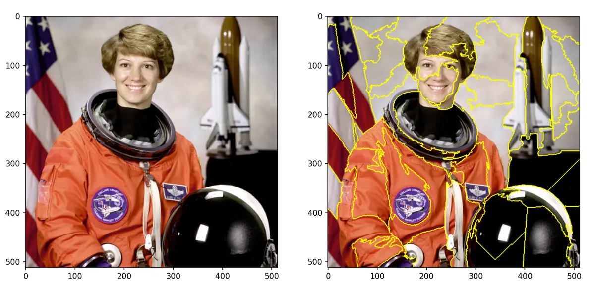
這種方法提供了一個影象,在標記部分之間具有突出的邊界。skimage.segmentation.mark_boundaries() 函式返回帶有標記區域邊界的影象。
我們將使用下面的程式碼來使用這種技術。
from skimage.segmentation import slic, mark_boundaries
from skimage.data import astronaut
import matplotlib.pyplot as plt

plt.figure(figsize=(15, 15))

astronaut = astronaut()
astronaut_segments = slic(astronaut, n_segments=100, compactness=1)

plt.subplot(1, 2, 1)
plt.imshow(astronaut)
plt.subplot(1, 2, 2)
plt.imshow(mark_boundaries(astronaut, astronaut_segments))
plt.show()
使用上述程式碼為以下技術獲得分割影象。
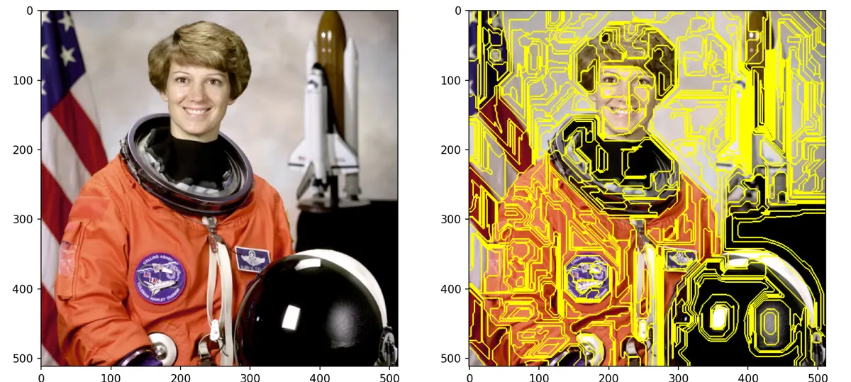
這種方法中的第二種技術是 Felzenszwalb 的分割。
在 Python 中 Felzenszwalb 的分割
Felzenszwalb 的分割使用快速的、基於最小生成樹的聚類來過度分割影象網格上的 RGB 圖片。在這種方法中使用畫素之間的歐幾里得距離。
Felzenszwalb 高效的基於圖形的影象分割是使用 skimage.segmentation.felzenszwalb() 函式計算的。
讓我們看看下面的程式碼來執行這種型別的分割。
from skimage.segmentation import felzenszwalb, mark_boundaries
from skimage.color import label2rgb
from skimage.data import astronaut

import matplotlib.pyplot as plt

plt.figure(figsize=(15, 15))
astronaut = astronaut()

astronaut_segments = felzenszwalb(astronaut, scale=2, sigma=5, min_size=100)

plt.subplot(1, 2, 1)
plt.imshow(astronaut)

# Marking the boundaries of
# Felzenszwalb's segmentations
plt.subplot(1, 2, 2)
plt.imshow(mark_boundaries(astronaut, astronaut_segments))
plt.show()
上面程式碼的輸出如下。
因此,我們通過在有監督和無監督分割方法中採用多種技術,成功地使用 scikit-image 模組在 Python 中執行了影象分割。